LAB 5.3: Global Solar Power Suitability
(Global Topography & Population Density) [
5.1,
5.2,
5.3, 5.4]
1
- Get GTOPO30
Purpose
The physical geography that pertains to
our problem of locating suitable locations for solar power generation
is going to be addressed using a global scale Digital Elevation Model
(DEM) dataset called GTOPO30. This dataset was derived from multiple sources
that were compiled mainly by Chris Verden at the EROS Data Center (EDC)
in Sioux Falls, SD. This dataset, as well as other NASA/USGS data products,
are available from the Land Processes Distributed Active Archive Center
(LP DAAC at EROS).
If you ever find yourself looking for geospatial data, EROS is usually
the best place to start.
The gridded population dataset for the
world we will be using was created using Waldo Tobler's pycnophylactic
interpolation algorithm, more about this gridded population dataset
can be found at National
Center for Geographic Information and Analysis (NCGIA, UC Santa Barbara).
The gridded population dataset, as well as numerous other global scale
data, are made available from by the Socio-Economic Data and Applications
Center (SEDAC)
at Columbia University.
Step
1 - Get GTOPO30
GTOPO30 is divided into 33 tiles. Each
tile is about 20 MB compressed, uncompressed each tile is about 80 MB.
How big would the folder get if we downloaded the each of the tiles accept
the 6 that cover Antarctica? (See Lab 5.3 Write-up).
Here is link to the main GTOPO30 webpage
if you are interested in seeing what all of the assembled tiles look like.
You can download the individual tiles form this website.
http://edcdaac.usgs.gov/gtopo30/gtopo30.asp
With Windows Explorer go to the lab5 folder
and create a new folder called "gtopo30".
Here is a link to the whole dataset resampled
and compressed with Arc Interchange format, and then WinZip (its about
2 MB compressed, ). Right-click, do Save Target As ..., save it in the
gtopo30 folder you just created.
GTOPO30
(resampled)
After you've saved it, unzip the file it
contains (gtopo30res.e00) into that same folder. Once you have extracted
the .e00 file, close WinZip.
Step
1.1 - Import the .e00
The GRID raster data format actually consists
of a folder with interlinked files, and another folder called info. But
you know what. Should you ever want to move an individual grid you need
to export it to a special kind of file that preserves the file structure
(the grid's folder of files, and the info folder with its files). To do
this you use Arc Interchange Format (.e00). This format makes the files
and folders into one file, and then use WinZip to compress the .e00. (See
Lab 5.3 Write-up)
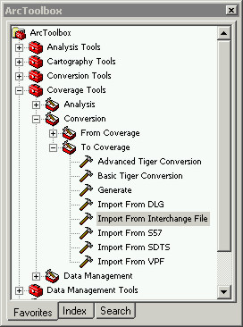
To import the grid from the .e00 file you
need to start Toolbox and go to Coverage Tools -> Conversion ->
To Coverage -> Import From Interchange File.
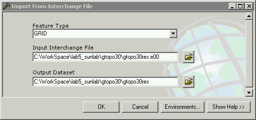
In the Import from Interchange File dialog,
set the Feature Type to GRID using the pull down menu, set the Input Interchange
File to the one you just unzipped (gtopo30res.e00), the Output Dataset
will default to the location of the .e00 file (this is what you want).
Click OK to import the grid.
If after the grid is written to the gtopo30
folder a window a open asking you if you want to build pyramid layers.
Click Yes. If ArcMap does not ask you to build pyramid layers this is
not a problem, the grid will open without it. Also, the pyramid layer
file (.rrd) can be deleted and recreated if necessary.
A pyramid layer is a file that contains
image statistics (called gtopo30res.rrd in this case) that tell ArcMap
how much to degrade the resolution when the data are displayed at a particular
scale so when you zoom in and out it can rescale the resolution based
on how much detail (how many pixels) you can see.
Right-click on the layer in ArcMap and
go to Properties, click on the General tab and look for the spatial dimensions
of the grid (rows, columns and cell size). (See Lab 5.3 Write-up)
Why am I asking you these questions? Because
you need to have an idea of how big (in spatial terms and in terms of
file sizes) the data you are working with are. This is important when
executing a project as you are now because in some cases the datasets
can get very large. Storage is not really an issue, but computer horse
power sometimes can be a bottleneck because the files become too big to
load efficiently. Also, there are limitations with the Windows operating
system as you will see.
Step
1.2 - Fix grid errors with a mask
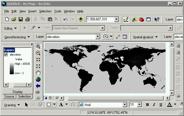
After you imported the gtopo30res grid and built
pyramid layers it will open in ArcMap
Upon viewing the grid some problems should be
apparent to you. First of all the oceans are all gray and there are white patches,
these are errors that have to be fixed. Use the Identify tool to click on a
few of these problems and see what the erroneous data values area. There are
more problems than meet the eye, but using the Identify tool will an idea of
the magnitude (the size) of the bad data values you need to fix.
We discussed NoData in the last lab, we are going
to fix the errors using a different technique this time. Reclassify is efficient
for grids that have a small number of data value(s). Reclassify modifies grid
cell values but with grids were only the difference, not the absolute magnitude
of the difference, is import it is suitable. Such is the case for Cloudiness
as a percentage, but with elevation this is not the case.
Step
1.2.1 - Look at the attribute table for gtopo30res
Elevation data are measured relative to sea level,
and the absolute magnitude of the difference between the elevation at different
points is an important property to preserve. Reclassify is not suitable for
elevation data for this reason, especially considering there are millions of
grid cells.
A quick look at the attribute table for the
gtopo30res grid will reveal the problem with the gtopo30res grid. This problem
is visually apparent when you look at in ArcMap, where's the elevation? The
data are there, but the default stretch of data values the ArcMap applies makes
all the variation indistinct.
Right-click on the gtopo30res layer, and choose
Open Attribute Table. Scroll down until you see a huge number under the Count
column (see below).
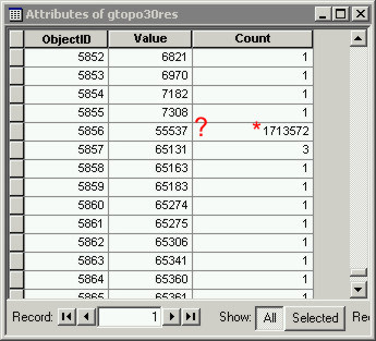
Value in the gtopo30res grid is elevation, and
the elevation is in meters. 7308 meter elevation is reasonable, much higher
than that is not. Also look at the Count next to obviously erroneous elevation
Value of 55537, that is a good indicator that these pixels need to be assigned
NoData. What do think 1.7 million pixels in this data set could be covering?
Ocean would be a good bet. This dataset covers the whole world, and the world
is about 70% ocean ... stands to reason. But all these pixels, as well as numerous
others, have a Value greater than 7308. (See Lab 5.3 Write-up)
All of the pixels with a Value greater than 7308
needs to get set to NoData in the gtopo30res grid. To do this we are going to
make a separate grid of just these erroneous values. This technique is called
masking.
Step
1.2.2 - Use Raster Calculator to make binary mask
The Spatial Analyst extension can do quite a
lot, the Raster Calculator in particular is a potent tool for generating and
modifying grids.
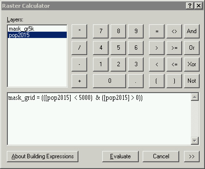
Go to the Spatial Analyst pulldown menu, start
Raster Calculator. In Raster Calculator
create a new grid that consists of all the data values we want to keep. Type
in a name for a new grid ("mask_grid" in the example shown below), and make
an expression that says, "create a new grid with all the pixels that have Value
less than or equal to 7308 in gtopo30res AND all the pixels with Value greater
than 0".
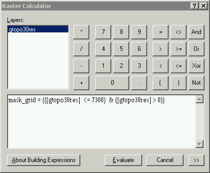
Raster calculator expression like this are called
"map algebra", basically the expression entered above is a logical operation
that translates as: "IF <= 7380 AND > 0, then TRUE, IF NOT <= 7380
AND > 0 then FALSE", True = 1 and False = 0. Every pixel in gtopo30res will
be tested with this expression, and every pixel in the new grid will be either
TRUE (1) or False (0).
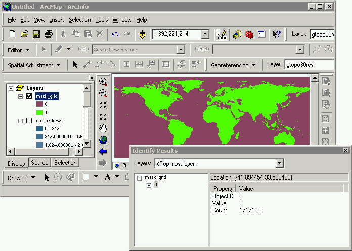
After click Evaluate, the new grid will be automatically
added to your ArcMap Layout.
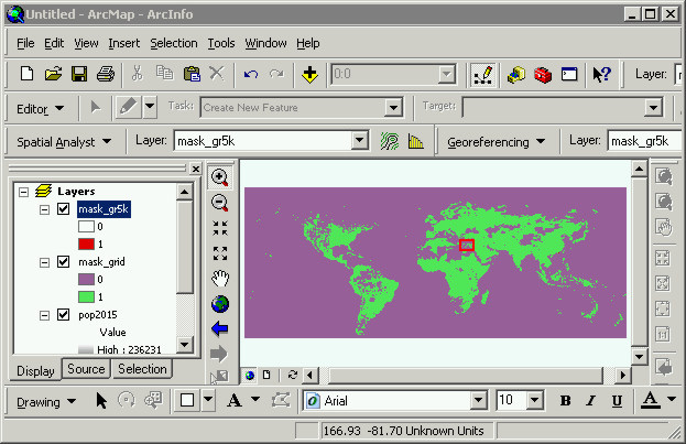
This is what is referred to as a "binary mask".
All the 0 pixels (purple in the screenshot below) are the pixels we observed
in the Attribute Table for gtopo30res that were need to change to NoData (this
is the equivalent of telling ArcGIS to ignore these pixels). The purple pixels
(0s) did not satisfy the map algebra expression you made (they were > 7308,
or < 1). The green pixels are all the good pixels that we want to use in
our analysis. Yes, it would be possible to put solar power generation facilities
in the water but this is not a practical consideration. (See Lab 5.3 Write-up)
Use the Identify to click in the purple somewhere,
all these pixels (all 1,717,169 on them!) are now 0.
Next we are going to reset all the 0s in the
binary mask to NoData.
Step
1.2.3 - Use Reclassify to reset mask 0s to NoData
In the step after this one we are going to multiply
the gtopo30res grid by the binary mask_grid. All the pixels that are multiplied
by 0 pixels in the mask grid will become NoData in the new gtopo30res grid (NoData
x any Value = NoData), and all the pixels that are multiplied by 1s in the mask
grid will keep their same value (1 x any Value = same Value). One trick we can
use at this point is to make all the 0 pixels in the mask_grid into NoData pixels,
this will preserve the original elevation values we want to keep as well as
make all the pixels we don't care about into NoData.
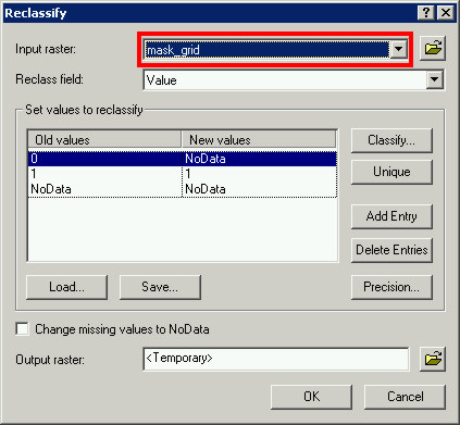
Go Spatial Analyst -> Reclassify. In the Reclassify
dialog set the Input raster to be mask_grid, under the New values column to
the right of the Old value 0 type in NoData. To the right of the Old values
1, type in a 1 under the New values column. Click OK.
After you click OK the reclassed mask_grid will
be added to ArcMap automatically, it will be called "Reclass of mask_grid".
Uncheck all the data layers underneath, only leave Reclass of mask_grid checked
on. Get the Identify tool and click in the empty space somewhere. What Value
do you get? Nothing, this is what is meant by NoData (its no 0 anymore in the
grid, its an empty cell with NoData in it). (See Lab 5.3 Write-up)
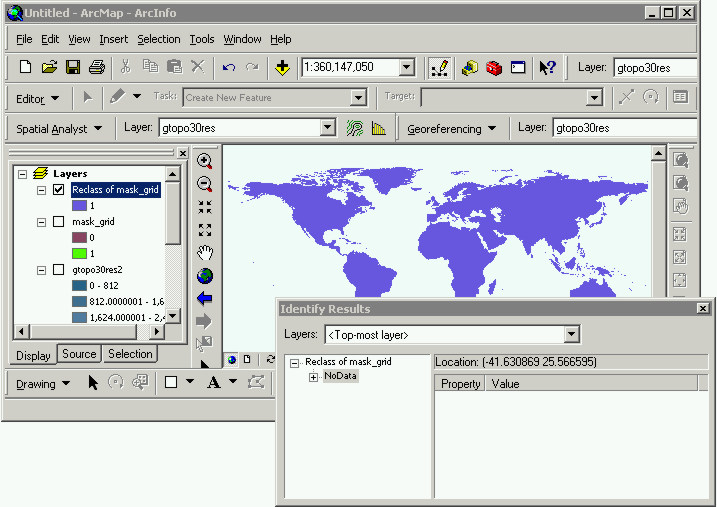
The mask grid now has 1s in all the pixels we
want to keep and nothing (NoData) in all the pixels we don't want to keep.
Step
1.2.4 - Apply the mask to gtopo30res
Start Raster Calculator again. This time we want
to create a map algebra expression to reset all the pixels with erroneous data
values and all the pixels with 0 values in the gtopo30res grid to NoData. This
will help with the analysis by telling ArcGIS which pixels in this layer are
irrelevant (NoData) and allow us to use an appropriate Symbolization Classification
based on the actual elevation values. By doing this we have preserved the absolute
magnitude of the differences between the pixels.
Remember the pixels that contain erroneous data
values in the mask grid are all NoData now, and the pixels with good data values
we've kept (these pixels were 1 in the mask_grid, so when we multiplied the
gtopo30res by mask_grid these values were unchanged).
Type in the expression shown below and click
Evaluate.
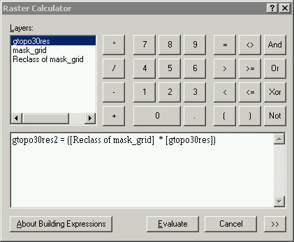
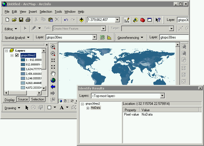
Click Evaluate and the new grid ("gtopo30res2"
in the example above) will be added automatically to ArcMap. Click on an Ocean
pixel or one of the pixels in a large inland lakes with the Identify tool, the
Value of the pixel you click on should no be NoData (which isn't really a value,
its NoData, its nothing).
The procedure you have just done, queried a grid
to make a mask and then applied the mask to a raster dataset to assign NoData
values is important for two reasons. First, it will allow ArcGIS to properly
scale the data values so when you display it you can see the full range of values
(as apposed to when you first loaded the grid after you imported it and it was
all black, white and gray). Second, by modifying the mask_grid to assign NoData
to all the pixels which had a Value of 0 we have reduced the number of pixels
that ArcGIS will have to analyses (it will automatically ignore NoData). Although
the computational savings is not that big relative to the map algebra expression
we will be using to evaluate Solar Power suitability, with higher resolution
(more rows columns) or with more data layers (if we included land use, distances
from major cities etc) this "data reduction" procedure would be significant.
Step
1.3 - Set the Coordinate System and Export the final elevation dataset
In the ArcMap window go up to View -> Data
Frame Properties, and make sure the Geographic Coordinate System is set to WGS
1984.
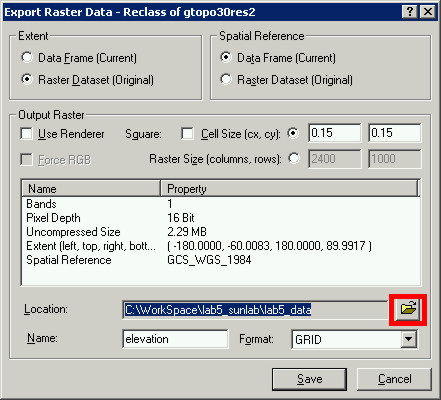
Right click on the "Reclass of gtopo30res2"
layer and do Data -> Export Data.
In the Export Raster Data dialog set the Spatial
Reference to Data Frame (Current), set the Location field to lab5_data (click
on the folder button and get it so you can see the lab5_data folder, highlight
it and click Add). Set the Name of the output grid to "elevation" (See below).
Click No when asked if you want to add it to
the ArcMap layout, we will be creating a new map for this dataset using one
of the others as a template.
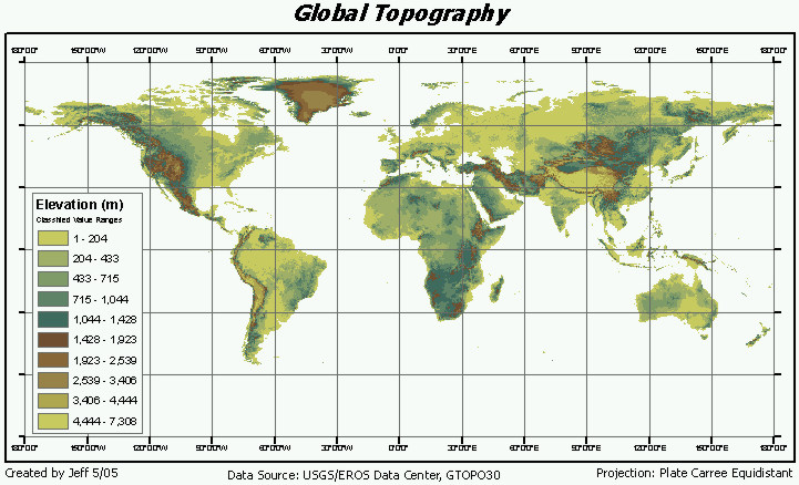
Step
1.4 - Make a map of global topography
As with the other data layers (TOA and Cloudiness),
I would like you to make a map using the elevation grid you just created. The
easiest way to do this is as you did before. Open one of the completed map layouts,
toa_map.mdx or cloud_mean_map.mdx, and do File -> Save As and name it "elevation
_map". Delete the old legend, and add the elevation grid you just created.
Elevation is different than the other two data
layers we've generated so far. Elevation, although technically it is "continuous",
in reality we don't think of it like that. When you see topography on a map
you are used to being able to visualize the dimensionality somehow. There are
a number of cartographic techniques for representing topography, we will address
this in Lab 6. For this map I simply want you to experiment with different visual
representations of the elevation dataset using ArcMap's Symbology options.
Right-click on the elevation dataset in the map
layout you just made, go to Properties -> Symbology. Try Classify and Stretch.
You will be learning more about Classify later when we cover Data Classification,
for now just make something that looks nice to you and you think represents
the global topography well.
Step
2 - Gridded Population
The physical environment (incoming radiation,
cloud cover, and topography) are one component, but in order to generate a map
of Solar Power suitability we need include somehow the human element. The most
basic human element to the problem is population, where people live. We could
include other socio-economic indicators for different states/countries/regions,
but for the sake of our global scale study all we want to accomplish is the
identification of areas for more detailed suitability studies.
SEDAC's website is a great resource for socio-economic
data. They also provide the gridded
global population density data (Gridded Population of the World GPW
v3: Future Estimates, 2015). I have downloaded the data already as sometimes
the java script that this page runs does not work correctly and can cause problems
with Internet Explorer's security settings (but it works fine with Mozilla Firefox).
Step 2.1 - Download global population data
With Windows Explorer go to the lab5 folder and
create a new folder called "pop"
Right-click here [ gl_gpwv3_pdens_15_bil_25.zip
] and choose Save Target As ..., save this zip file to the pop
folder you created.
Unzip the four files it contains (glds15ag_beta1.bil,
glds15ag_beta1.hdr, glds15ag_beta1.blw, and glds15ag_beta1.stx) to the pop folder
you just created. This will take a while, its a big file. Be patient.
Once the files are done extracting close
WinZip and look at the files in the pop folder. (See
Lab 5.3 Write-up)
Step
2.1.1 - Look at the data file and its header
This raster dataset is close to the limit of
what ArcGIS can handle and what the Windows operating system can deal with efficiently.
Also, these data are 32-bit. This means that both the range of possible values,
and the size of the data file is huge. There is really no need at all for population
density data to be represented with 32-bit values, but that's what we've got.
I have created the header file for you so you
don't have to wade through the mess that is called "FGDC standard metadata"
to find all the parameters, I have also added a file called a "statistics file"
that has the .stx extension, and another file that summarizes the grid plotting
parameters. These two file are used by ArcGIS to read the data file more efficiently,
they contains the min/max, and other summary statistics. An .stx file is necessary
for properly loading grids this large, with smaller sized grids (like monthly
cloudiness) ArcGIS can calculate these values efficiently.
I want you to look at is the resolution of this
dataset (both extent and pixel size), as well as the file size. Open the header
file (glds15ag_beta1.hdr) that was unzipped with the .bil file.
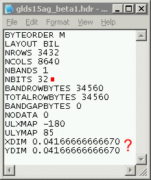
The spatial units of this dataset is decimal
degrees, how big is a pixel (in degrees) if it is .0417 x .0417 decimal degrees?
How many pixels are there in this dataset? (See Lab 5.3 Write-up)
Step
2.1.2 - Load the bil file and set the projection
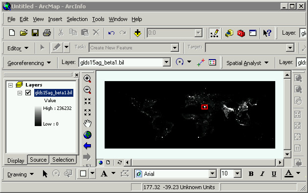
Add glds15ag_beta1.bil to an empty ArcMap layout,
you can either do this using the Add Data button or drag it in to ArcMap from
Windows Explorer.
If ArcMap prompts you for Pyramid Layers, click
No. Go up to View -> Data Frame Properties and set it to WGS 1984.
Errors in datasets like this are difficult to
detect. Like the data values of GTOPO30, these data have values we can think
of in real terms (sort of). Elevation is more intuitive than Population Density
for sure, but we can still think about it in realistic terms.
Step
2.2 - Look at the data values with the Identify tool
The data values in the in glds15ag_beta1.bil
are population density (people per square kilometer). Could there be more than
100,000 people living in a square kilometer? No, not really, but this dataset
is the result of a complicated statistical modeling technique (pycnophylactic
interpolation) and is based on extrapolating from past growth rates.
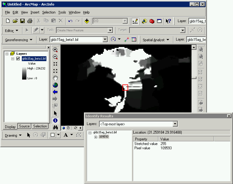
In ArcMap zoom in until you have Cairo, Egypt
in the map window. Use the Identify tool to click around and get an idea of
the range of data values. In the screenshot below I identified a pixel that
is projected to have a population density of more than 100,000 people per square
kilometer by 2015. It is true that Cairo is the most densely populated city
in the world, but this value is way out of proportion relative to other densely
populated urban regions (probably due to the method with which the growth rates
were extrapolated).
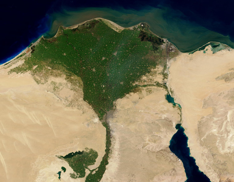
For reference here is a MODIS satellite images
of this area. This image was acquired by one of NASA's Earth Observation Satellite
(EOS) called Terra on 2/2/2003.
When you are doing clicking around Cairo, and
trying to contemplate how nasty its going to be there in a decade, covert the
.bil to a GRID. (See Lab 5.3 Write-up)
Step
2.3 - Convert the bil to a GRID
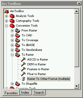
To convert the .bil file to a GRID start Toolbox
and go to Conversion Tools -> To Raster -> Raster To Other Format (multiple).
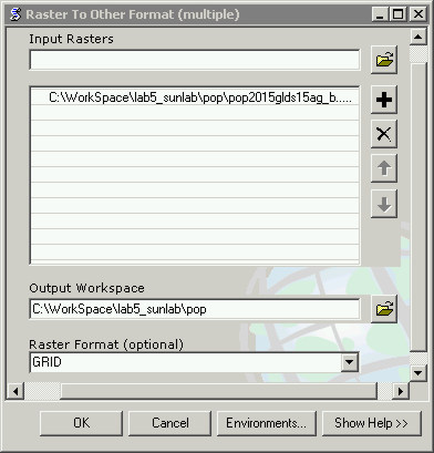
In the Raster to Other Format (multiple) dialog
set the Input Rasers to the .bil file, set the Output Workspace to be the pop
folder, and the Raster Format as GRID. Click OK.
Add the pop2015 grid to ArcMap and get rid of
the .bil file (right-click on the glds15ag_beta1.bil in ArcMap and choose Remove).
Step
2.4 - Extract the pixels that cover the most densely populated areas in the
world
The raster data format permits quick processing
("raster is faster"), so searching through 3432 x 8640 pixels is a relatively
quick procedure.
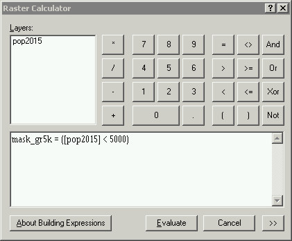
Go to Spatial Analyst -> Raster Calculator
to make a map algebra expression that says,
"make a grid with all the pixels in pop2015 with Value less than 5000" (see
below).
This expression will create a new grid with all
the pixels being either 0 (false) and 1 (true). Raster Calculator will test
every pixel's Value and determine if it is either less than 5000, in which case
it is true (1), or if it is greater than or equal to 5000, in which case it
is false (0).
The new grid (mask_gr5k) will be automatically
added to ArcMap, but it written to the Windows temporary folder ( C:\Documents
and Settings\user\Local Settings\Temp ). To make a copy of this grid go to Data
-> Export data. Add the newly exported grid to ArcMap, and the Remove the
old one. (See Lab 5.3 Write-up)
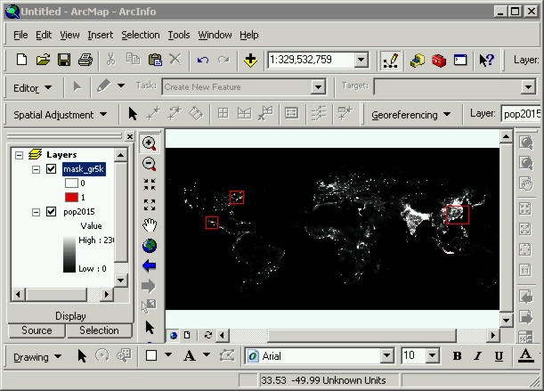
Right-click on the grid (mask_gr5k) and choose
Properties, go to the Symbology tab and change the 0s to red (the pixels with
Value geater than or equal to 5000) and set the 1s to hollow so you can see
though to the layer underneath. The red mask_gr5k pixels should now be on top
of pop2015.
Step 2.4.1
- Examine the global population density "hot spots"
The screenshot below shows some massive urban
conurbations with red boxes around them. Some of these areas should be familiar
to you from your extensive studies of world geography. At least you should be
familiar with the Western Hemisphere (Washington-Baltimore, and LA, SF, and
Mexico City), there is also a red rectangle around China. If you are not familiar
with the great cities of the world, add the Cities shapefile. This shapefile,
as well as numerous others, can be found in the folder where ArcGIS stores the
datasets it uses for the World map templates ( C:\Program
Files\ArcGIS\Bin\TemplateData\World ). I have also included it with lab5_data.zip
in case you cannot access this folder.
There are only about 4,600 pixels out of this
entire dataset that meet the >= 5000 criterion, and most of them are in China.
Although this dataset is a statistical model prediction for a decade from now,
the population density of China is already difficult to comprehend by our standards
of living.
Now that you've familiarized yourself with the
dataset a little bit we are going to simplify it a bit by removing these extreme
values.
Step
2.4.2 - Mask outlier pixels
In order to "fix" the pixel values in this dataset
we are going to create a series of binary masks from the pixels with 0 <
Value < 5000.
Start Raster Calculator again, and make an expression
that says, "make a new grid with all the pixels in pop2015 that are both less
than 5000 and greater than 0".
After you click Evaluate the new grid will be
automatically added to ArcMap and as before it was written to the Windows temp
folder, to keep a copy right-click and do Data -> Export Data then remove
the old one. Move mask_gr5k over the top of mask_grid and zoom in to Cairo where
we observed the collection of unbelievably high valued pixels before.
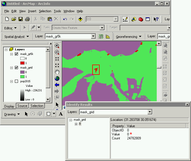
If you check and uncheck the mask_gr5k grid on
and off you will see that these pixels are now 0 in mask_grid. Get the Identify
tool and click on the patch of pixels that we masked using the map algebra expression,
set the Layer field in the Identify dialog to be mask_grid. The Value of all
of these pixels in mask_grid (show in red in the screenshot below) are now 0.
Step
2.4.3 - Apply the mask_grid to pop2015
Go to Spatial Analyst -> Raster Calculator
and make an expression that will create a new grid by multiplying original pop2015
grid by the mask_grid. All of the pixels that have a Value of 0 will change
all the same pixels in pop2015 to 0.
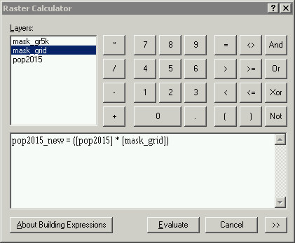
The new grid, "pop2015_new" in the example above
will be added to ArcMap automatically.
Step
2.5 - Look at the masked grid
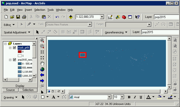
Lets look at another populated place more close
to home. Zoom to full extent and zoom in the Washington-Baltimore area (shown
in the red rectangle below).
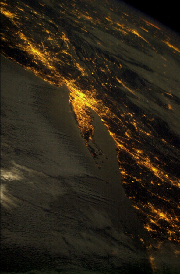
The image below shows this area from space. It
was acquired at night from the International Space Station on January 2003.
The view is oblique pointing westward, it shows the wall-to-wall urban area
that is New York and Long Island.
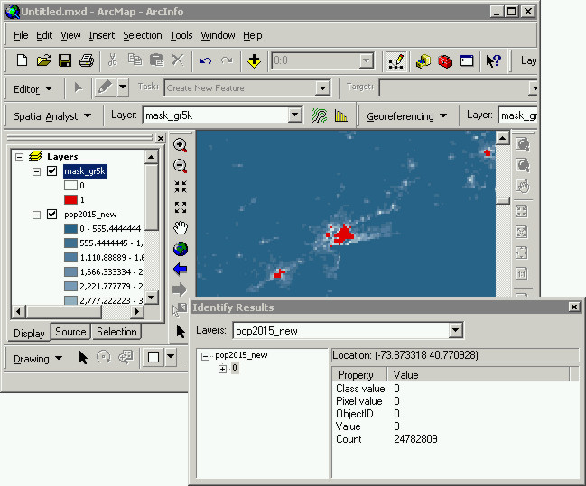
We have a problem now, albeit a self created
problem. Move the mask_gr5k layer up so it is on top of pop2015_new. Get the
Identify tool and set the Layers field to pop2015_new. Click on that big red
blob that is New York, Long Is(shown in the screenshot below). The pixels in
this area now have a Value of 0, lets fix this.
Step
2.5.1 - Fill in the masked pixels
The mask_gr5k grid has all the pixels from the
original population density grid set to 0 that were not at least 5000, all the
pixels with Value greater than 5000 are set to 1.
We are now going to add the values from the mask_gr5k
back to fill in all the pixels we set to 0 before, but we are going to make
them all 5000. To do this first we will do a Reclassify on mask_gr5k and make
all the pixels with 0s into pixels with a value of 5000.
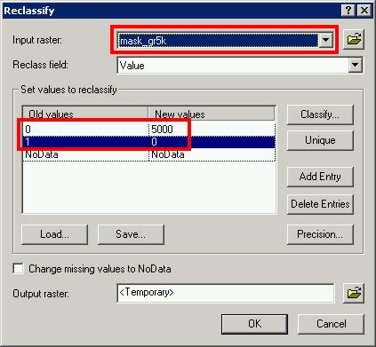
Go to Spatial Analyst -> Reclassify, set the
Input raster to mask_gr5k, change the New value to the right of 0 to 5000 and
change the New value to the right of 1 to 0. Click OK, the results will be added
to ArcMap automatically and called "Reclass of mask_gr5k"
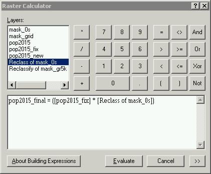
Go to Spatial Analyst -> Raster Calculator.
Make a map algebra expression that says, "create a new grid called pop2015_fix
by adding all the Values of the pixels in Reclass of mask_gr5k to those in pop2015_new"
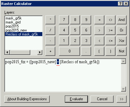
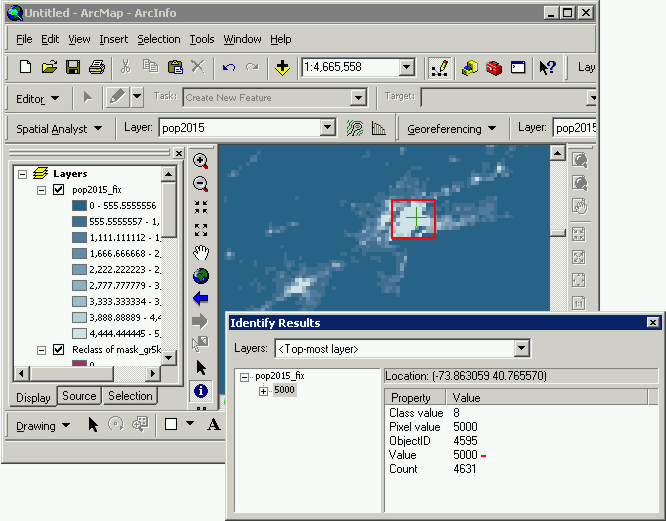
The new grid, "pop2015_fix", should be added
to ArcMap automatically. Check to make sure it worked by clicking with the Identify
tool on the New York, Long Island blob. It should now return 5000.
Almost done, that last step is the make a mask
that will reset all the 0 pixels to NoData.
Step
2.6 - Mask 0s with NoData
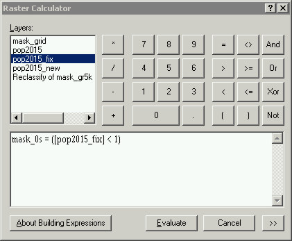
Go to Spatial Analyst -> Raster Calculator,
make a map algebra expression that says, "make a new grid called mask_0s with
all the pixels that are less than 1 (0) in pop2015_new".
Name the new mask "mask_0s" and use the input
grid "pop2015_fix", and < 1 to get 0.
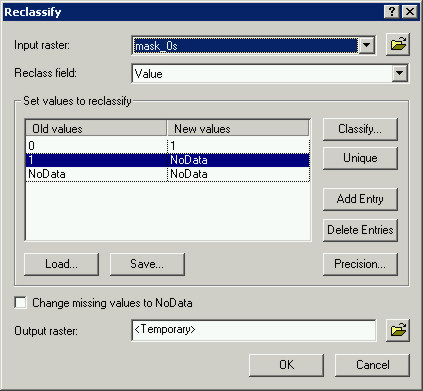
Use Spatial Analyst -> Reclassify to modify
the Value of mask_0s pixels. Put a 1 in the New values column to the right of
0 in the Old values column, and type in NoData next to the 1 in the Old values
column. Click OK and the reclassed grid ("Reclass of mask_0s") will be added
to ArcMap automatically.
Spatial Analyst -> Raster Calculator. Make
a map algebra expression that says, "make a new grid called pop2015_final by
multiplying pop2015_fix by Reclass of mask_0s"
Step
2.7 - Export final grid
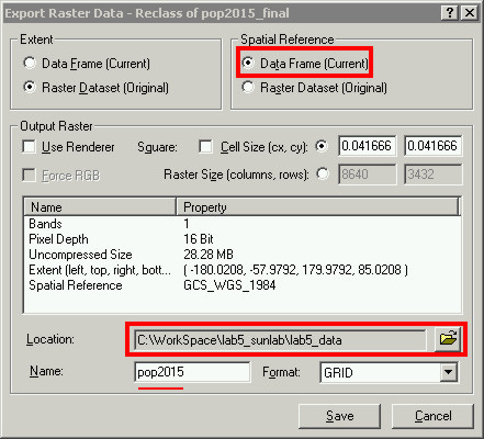
Right-click on Reclass of pop2015_final and do
Data -> Export Data.
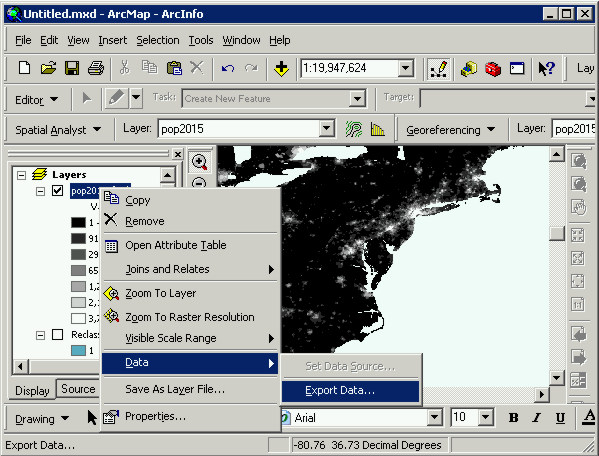
In the Export Raster Data dialog, set it to use
the current projection, set the output folder to be lab5_data, and name
the final grid "pop2015". The click Save, and click No when asked if you want
to add it to the map. We will be making another map using this dataset you have
just created.
Once you've exported the global population density
grid to the master data folder (lab5_data). Close ArcMap, and clean up the mess.
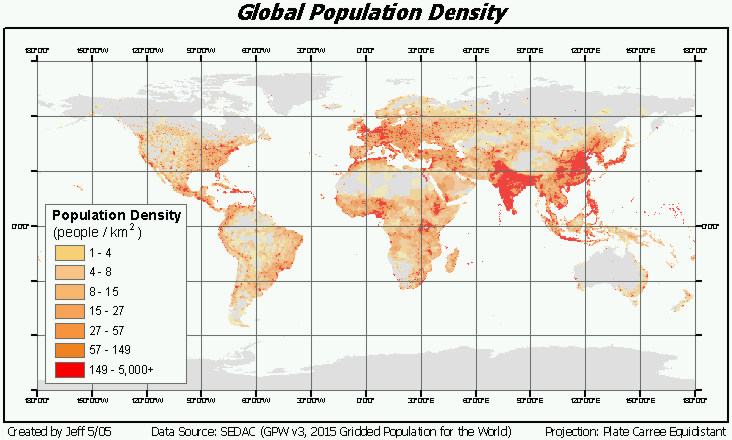
Step 2.8
- Make a map of Global Population Density
The global population density grid you've just
created is the most complicated raster dataset we will have a chance to work
with this quarter. The data values are ratio (people/area) and they were derived
using extrapolated growth rates and estimated over space using a sophisitcated
interpolation technique. Basically, this map should reflect the work that has
gone in to it.
As you did before, open one of the other map
layouts and do Save As ..., save the new map layout. This will make all four
of your final maps consistent: same font, north arrow, projeciton, graticule,
legend placement etc. If all of your maps are differnet I want you to change
this, choose one layout format you like (your "signature" map style) and stick
with it for all of them. Lab 5.4 will be where we perform the analysis using
the data we have created and produce our final maps, we will also be creating
a webpage describing each data layer we used, the basic data manipulations and
our final results. Being consistent between each of the maps is important.
For the Global Population Density map add the
county shapefile in the background, and all pop2015 on top of it. Use Classified
to add the color symbolization. For the map below I used Quantiles with 8 classes
(but deleted the 1st color as it was visually too close to distinguish from
the next). This is your chance to earn your "carographic license".
Step
3 - Clean up
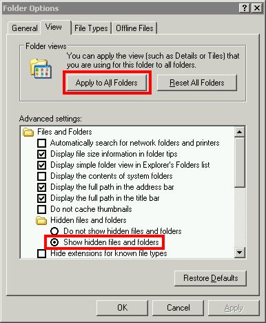
In Windows Explorer go to C:\Documents and Settings\user\Local
Settings\Temp. You make have to change the settings of Windows Explorer to allow
you to see this folder, sometimes it is a "hidden folder". Why I don't know.
To be able to see it go Tools -> Folder Options, and click on the View tab,
and then click next to "Show hidden files and folders", then click Apply (ignore
any warning messages, if there are any). Then click the Apply to All Folders
button, and click OK.
Now go to C:\Documents and Settings\user\Local
Settings\Temp
In that folder you will see all kinds of ArcGIS
droppings. You can delete all these files, some times these files can cause
headaches when you are working interatively through a problem because they get
mixed-up with other files. Its best to keep a clean ship.
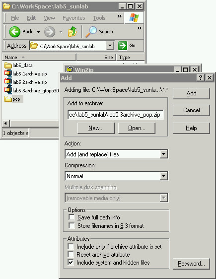
In Windows Explorer, go to C:\Workspace\lab5\pop,
in this folder get rid of the original glds15ag_beta1.bil file and all of the
associated files. This you should do, that bil file is pretty big and its worthless.
We have what we need in lab5_data. After you've deleted the .bil file, go up
one level so you can see the pop folder, right-click on it an choose Add to
Zip ... and zip the whole folder, call it "lab5.3archive.zip"
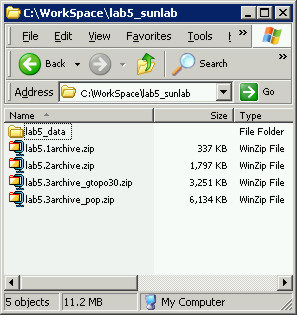
After you've backed up the pop folder with WinZip,
delete the pop folder. All you have left should be the master data folder and
four .zip files.
Deliverables
for Lab 5.3 (Global Topography, Population Density)
Map of Topography. We will be making
a map of Population Density after we discuss Data Classification next week in
lecture.
Lab
5.3 Write-up
recreated by jeff
5/5/05, with help from julie,
last updated 5/05