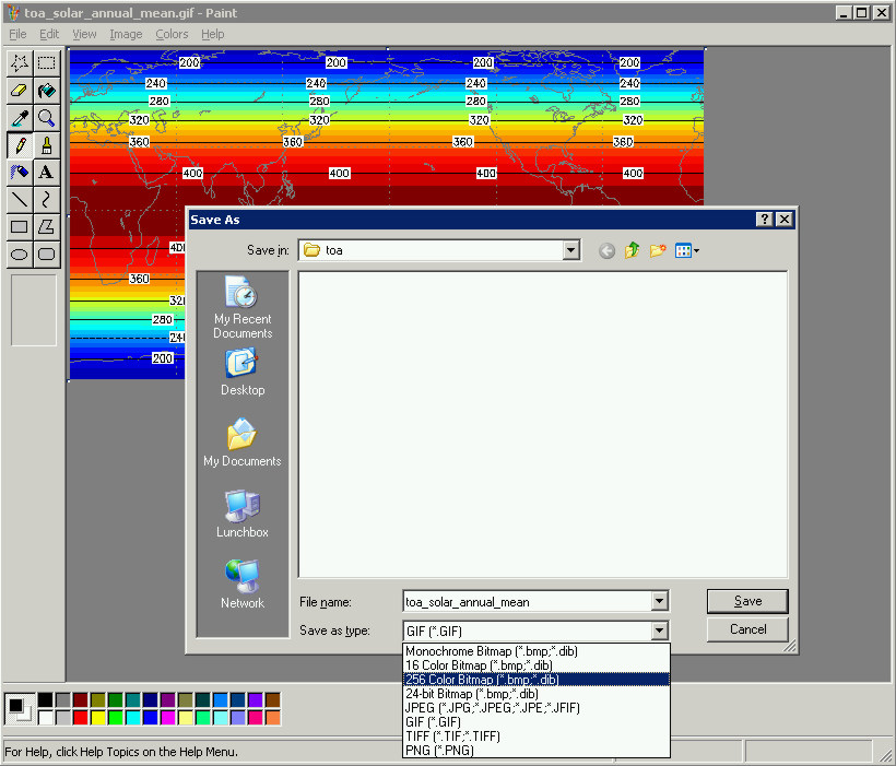
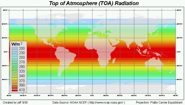
Many datasets you see on the web (or printed on paper maps) you cannot easily get as actual geospatial data. Either the original data used to compile the map are gone, the person who created the map is unreachable, or the image presents the spatial distribution of a complex distillation of multiple data layers, models or equations. This last case is where we find ourselves now. TOA (Top of Atmosphere) solar radiation although it seems like a straight forward problem, in reality its not that simple. We are going to use a gif image file to generate a dataset that represents TOA.
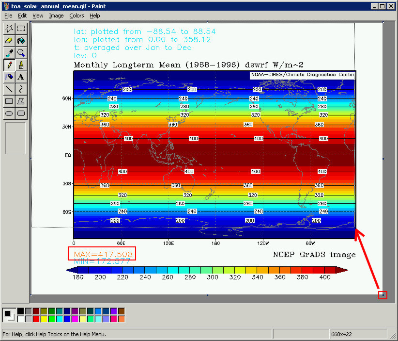
We will not need the extraneous information in the collar of the gif image. Once you have made a note of the useful information (coordinate reference information, Max value etc), use MS Paint to crop the image. (See Lab 5.1 Write-up)
Cropping an image using MS Paint requires five steps, these steps are illustrated in the following screenshots.
1) In the lower-right of the image grab the black block that represents the image corner. Move the corner of the image up and to the left so the image corner is inside the color part of the image about half a centimeter from the right side, and a centimeter or two up from the bottom. There is no need to be precise with this, move it to approximately the location shown in the screenshot below.
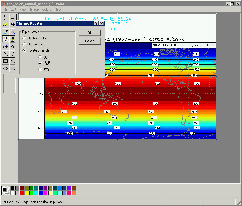
2) Go up to Image -> Rotate, select Rotate by angle, and choose 180.
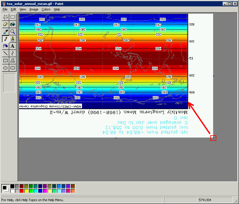
3) In the rotate image, grab the black block on the lower-right corner again and move the corner up and to the left. Approximate the location shown in the screenshot shown below.
4) Go up to Image -> Rotate, select Rotate by angle and 180 again so it is North up again.
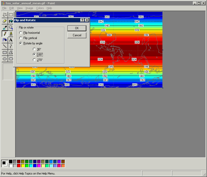
5) Go up to File -> Save As ... be sure to retain the original "bit depth", 8-bit (256 colors), not 24-bit (16 million colors). Save the image as a Windows Bitmap (.bmp)
Step 3 - Change the project of the countries dataset
Start ArcMap with an empty layout. Add the continent boundaries. All of the datasets used by ArcGIS to make the predefined map layouts can be found in C:\Program Files\ArcGIS\Bin\TemplateData\World
Change the Symbology for the continent shapefile so all you see are the lines (make the countries empty/hollow).
Next go to View -> Data Frame Properties. Under the Coordinate System tab go to Predefined -> Projected Coordinate Systems, and highlight Plate Carree. With Plate Carree highlighted, click the Modify button to the right.
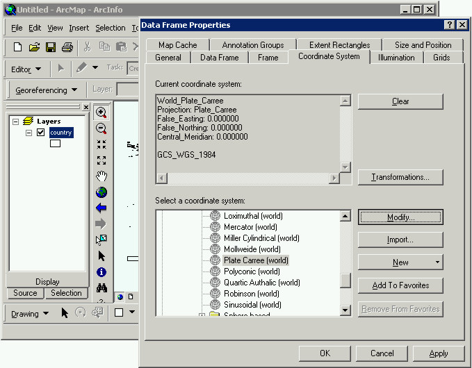
You need to get the continent boundaries to match those of toa_solar_annual_mean.bmp in order to proceed with the next step of giving the image file real world coordinates. Basically what you need to do is shift the projection's central meridian 180 degrees.
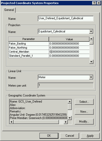
After you click Modify the Projected Coordinate System Properties dialog will open where you can change the Central Meridian. To do this just type 180 in the Value column next to the Central_Meridian row.
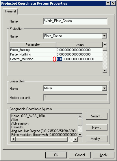
Click Apply, then OK to close Projected Coordinate System Properties dialog. Then click Apply and OK again to close the Data Frame Properties dialog. The continent boundaries should re-center themselves along the 180th meridian.
Add toa_solar_annual_mean.bmp to the same ArcMap layout.
Turn on the Georeferencing toolbar (go to View -> Toolbars -> Georeferencing).
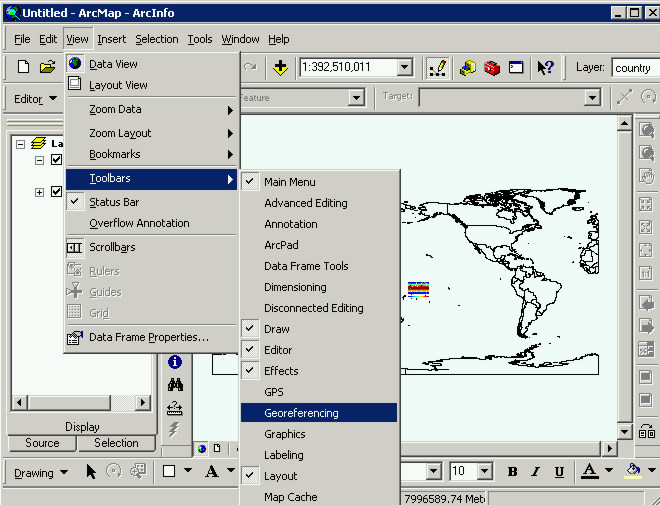
This will open a new toolbar floating around, snap it into the top part of the ArcMap window under the Editor pulldown button. To do this click and hold down the two little vertical bars on the left most side of the floating Georeferencing toolbar. Once you've got a hold of it drag it up there and it should snap itself in. You can move all toolbars this way.
Next to the Georeferencing pulldown menu button there is a field with the source Layer, make sure it says toa_solar_annual_mean.bmp.
Right-click on the toa_solar_annual_mean.bmp layer in ArcMap and choose Zoom To Layer. It might be helpful to maximize ArcMap to give yourself as much room to work as possible.
Click on the Add Control Point button (it has a diagonal line connecting a pair of red and green crosses). After you do this the cursor will turn into a cross, but if you move the cursor out of the editable area it will turn back to normal and you can select different tools (like the pan, and magnify tools).
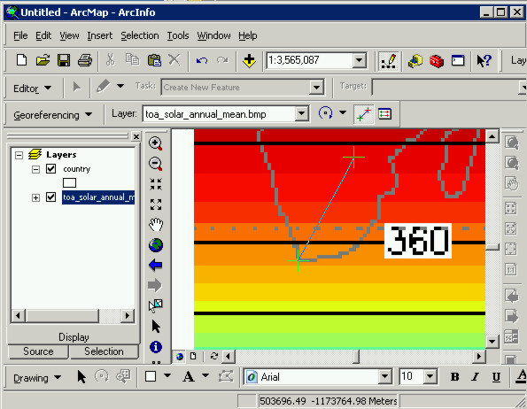
Zoom in to southern tip of Africa in toa_solar_annual_mean.bmp by just clicking (the image units are difficult for ArcMap to translate, if drag-out a box it might get lost). Click 5-6 times until you are in far enough to visually see the width of the line of pixels that comprises the southern most tip of Africa as is shown in the screenshot below. Get the Add Control Point cross hairs cursor again and add a point. After you click the cursor cross hairs will have a line attached to it.
The "from" point is where you just clicked on the tip of Africa in the bmp image. You need to get to that place (the Southern tip of Africa) on the continent boundary shapefile and add the ending "to" point. To do this zoom to full extent. You should see the continent outlines and the rainbow colored bmp in the middle of them somewhere, select the magnify tool again and zoom in to the southern most tip of Africa in the continent boundaries shapefile. You can drag-out a box this time, or click to zoom in, whatever suits you.
Once you have zoomed in to where you can see the vector outline of the southern tip of Africa, select the Add Control Point button again. Notice that the line is pointing back in the direction of the original "from" point. Click on the southern tip of Africa with the Add Control Point cross hairs.
Zoom out to full extent again, or you can right-click on the data layer and select Zoom To Theme.
All that one from-to Control Point did was move the bmp over, now add another Control Point to stretch it out, but this time go up to the eastern tip of Iceland.
After you add the control point from Iceland on the bmp image and Iceland in the continent boundaries dataset, you should add another control point. The Eastern (US facing) side of Japan is a good choice. That should be good, but if you boundaries don't line up you might been to add another point (the southern tip of South America would be a good choice).
Once you've added that last point, inspect the fit of the warped bmp to the continent boundaries. Remember that "good enough" in this case is a distance approximately about three times the width of one of the pixels constituting the lines of the countries in the bmp image. If you're in doubt ask me to come look at it.
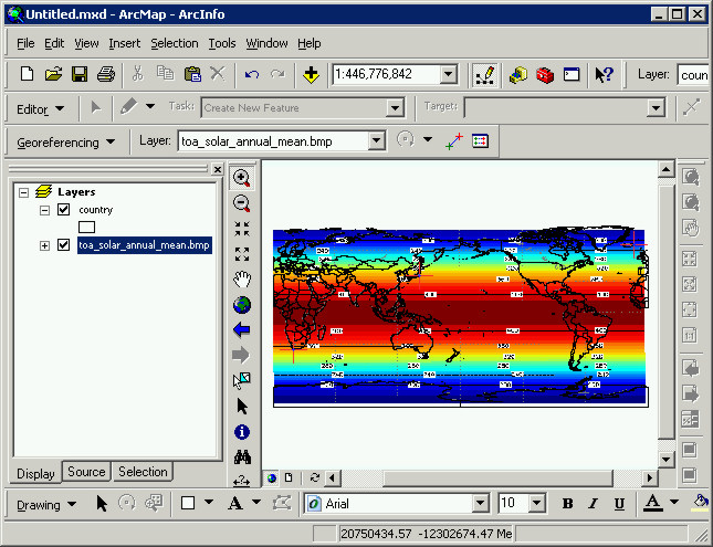
If the boundaries visually agree you're done and you should have something that looks like this.
If for some reason you would like to redo a point, you first should remove that point from the Link Table.
Step 4.2 - Look at the Link Table
View the actual control points you just created. Click on the View Link Table button which is beside the Add Control Point button at the top of ArcMap.
Click the Save button on the Link Table window once you have it open. Save these points in the lab5_data folder. The link table is a text file that you can Load again should you need to remove and/or redo some points later and resave the Link Table. You shouldn't have to redo this, but its good to keep track of these kinds of files.
To remove one of the points highlight it, and the click the X button.
You can close the Link Table if it is in your way and re-open it by just clicking on the button again. If you do modify the links though, be sure to Save the Link Table again so you can Load it later if necessary.
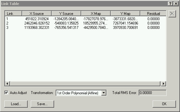
Your numbers will be different then the ones shown in the screenshot above. The coordinates shown Link Table are the coordinate pairs used to transform the bmp image to real world coordinates. A Control Point consists of a from point (x, y coordinate on the bmp) and to point (x,y coordinate on the continent boundaries dataset). These coordinate pairs are used to calculate the slope of the formula for a line (y = mx +b), the formula for a line is a "1st Order Polynomial (Affine)". This formula is used to convert every input x,y coordinate (every pixel) in the bmp image to a new output coordinate.
You can add more points and do 2nd or 3rd order. With each higher order polynomial you will introduce different kinds of nonlinear distortions to the equations that transforms the image to the real boundaries. A 2nd order is exponential, meaning it'll make curves, and 3rd order is quadratic, meaning it'll make parabolic shapes.
In the case where the image you want to rectify (or "warp" in GIS speak) is already planar, higher order polynomial transformations are not helpful because the image is already "flat". (See Lab 5.1 Write-up)
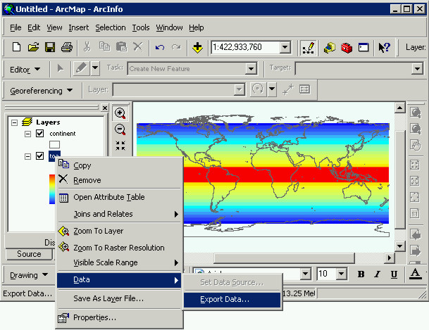
After you've georeferenced the image file to the continent boundaries do Data -> Export Data to make the coordinate transformation permanent.
Right-click on the bmp data layer, go to Data -> Export Data. This will convert rectified bmp image into a grid. GRID is technically a ESRI raster (image) data structure, but its also a "grid" in the normal sense of the word. It consists of rows and columns of pixels (or cells).
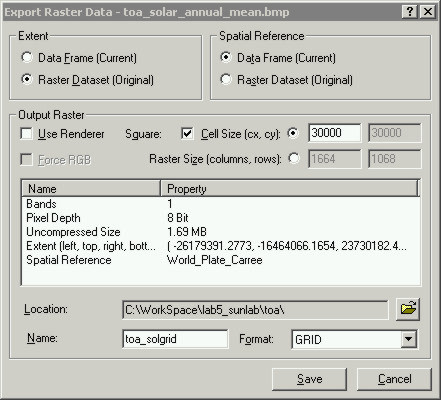
In the Export Raster Data dialog that opens, select Data Frame (Current) for the Spatial Reference, check on Cell Size and set it to 30000, change the Name to "toa_solgrid", then click Save and Yes so that it will be added to the map layout.
After the rectified grid is added to the ArcMap layout, and you've saved your Link Table, you can remove the bmp image (right-click, choose Remove).
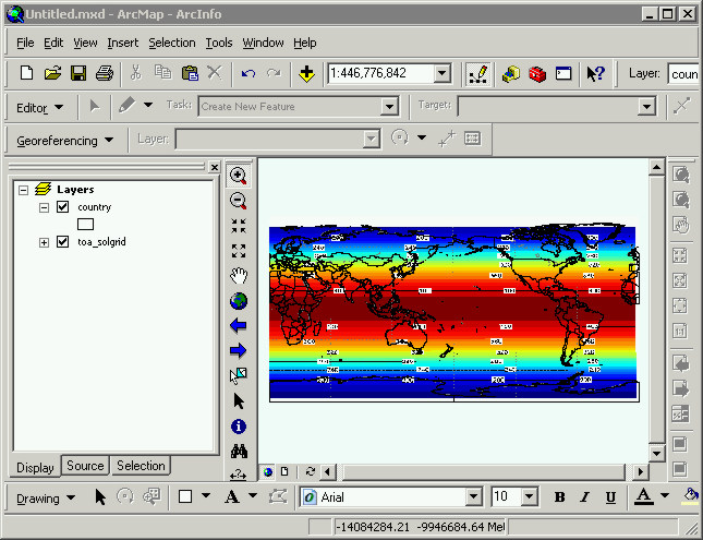
What you have so far should look like the following. Instead of the rectified bmp, you have a grid that as the same coordinates as the continent boundaries.
A bmp and the ArcGIS image format known as "GRID" are technically both rasters, but the GRID format is different because it stores geospatial information and ArcGIS can use the data values contained in the pixels for analysis.
Step 5 - Resample, convert to points, edit
Step 5.1 - Resample the TOA grid
Although it might be desirable in some cases to preserve as much resolution as possible, in this case it isn't. All we want is a global scale TOA dataset, but in order to get this we need to remove the artifacts introduced by the continent boundaries, the text and lines in the original image. First resample the image, this will degrade the resolution by making the pixels (cells) a lot bigger.
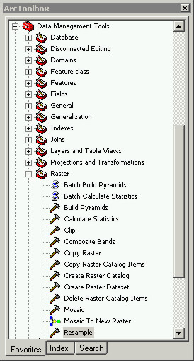
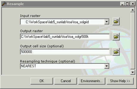
To resample the TOA grid created start to Toolbox, go to Data Management Tools -> Raster -> Resample. In the Resample dialog specify the Input raster as the one you just made, toa_solgrid. Name the Output raster "toa_solgr500k" and set the Output cell size to 500000. Click OK, and if the resampled grid doesn't get added to your map automatically add it.
 |
|
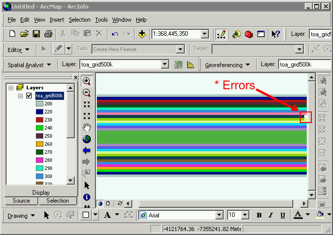
There should be an new grid with errors (gray pixels, black pixels, and white pixels). These errors are the text and lines from the original image. The resampled grid is barely recognizable, but this is what we want. We need to fix the artifact/error pixels, to do this we need to first make this grid into points.
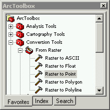
Step 5.2 - Make the grid to points
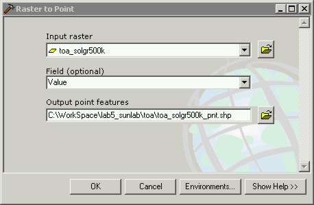
Make the resampled grid (toa_solgr500k) into points using Toolbox, Conversion Tools -> Raster to Point.
In the Raster to Point dialog set the input as the resampled grid, and name the output "toa_solgr500k_pnt.shp", and click OK. The new point shapefile should get automatically added to ArcMap.
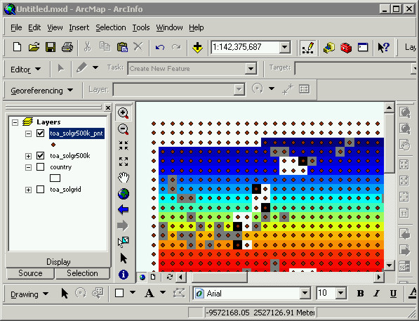
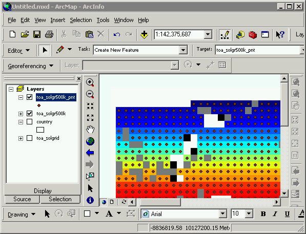
Now you have a grid of points that are spaced 500 kilometers apart and it should look like this.
 \
\
Now we need to fix the errors.
The points where there are white, black and gray cells underneath we need to get rid of. The attribute that the points have retained from the conversion, the one that associates them with the TOA statistic on the original gif map, is GRID_CODE. Find the GRID_CODE values of the points we need to get rid of using the Identify tool, click on the points where you see white, black and gray pixels underneith. Write down on a piece of scratch paper, or just remember, their GRID_CODE values. (See Lab 5.1 Write-up)
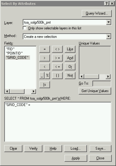
Click on the Editor button, and from the pull down choose Start Editing. Query toa_solgr500k_pnt.shp for the GRID_CODE values we want to get rid of. Go up to the Selection pulldown menu at the top of ArcMap, and start the Select By Attributes dialog.
Put in the artifact GRID_CODE value in the query and click Apply.
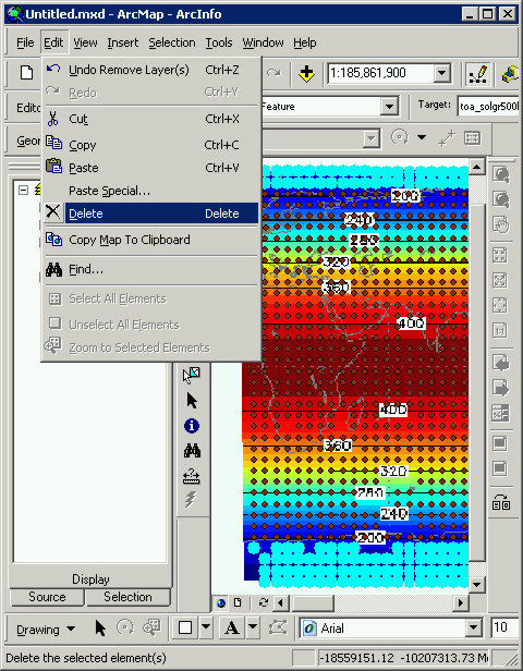
The selected points should be highlighted now, with these points selected go up to the Edit pulldown menu along the top of ArcMap, and pull down to Delete.
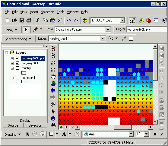
Repeat this procedure for the other erronious GRID_CODE values and delete them as well. After you have deleted the unwanted points with the erronious GRID_CODE values your grid should look like the following. All the artifact cells do not have any points.
Go up to the Editor pulldown menu and do Save Edits. Saving the map is not the same as saving your edits.
The grid of points (called a "lattice" in GIS terminology) are all correct with respect to the grid underneith. Now we need to fill in correct points in the empty spaces. (See Lab 5.1 Write-up)
Step 6.1 - Copy paste points to fill in the gaps
Delete the points that represent values that are too low to even consider for Solar Power. Points north and south of the line demarcating 200 W/m^2 are too low.
Uncheck the resampled grid, and check on the higher resolution version (toa_solgrid) so you can see where this line is.
With the Edit Tool (black triangular arrow), click and hold in the white space beside the beginning row and draw-out a box over the top two rows of points (North of the 200 line), hold down Shift and do the same thing for the bottom rows of points (South of the 200 line). With the points representing values less thatn 200 W/m^2 go up to Edit and pull down to Delete (or just push the delete key).
Check off the full resolution TOA grid, and check on the resampled TOA grid (the one that matches the resolution of your points). Click on the Editor button and from the pulldown menu choose Save Edits.
What you are now doing is called "manual editing", its part of GIS that everyone has to know how to do at some point but unfortunately it takes quite a bit of practice to get good at it. That is why we are starting with points, lines are much harder, and polygons are harder still. The specifics of what we are doing are important, but the digital dexterity you will be developing is important. Although it is important to be correct, more often then not being quick is equally as important. Being able estimate how long it takes you to do specifically defined tasks like this is a profitable skill as well; knowing how long it'll take you to make something is one of the main difference between a professional and a novice. Time yourself at this. (See Lab 5.1 Write-up)
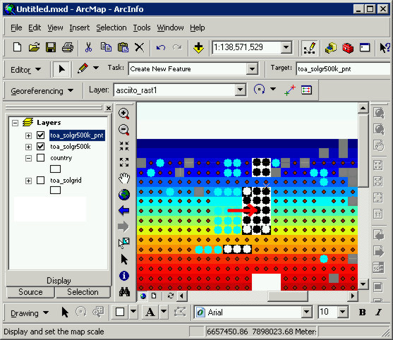
Zoom in to a portion of the editable area, and maximize ArcMap to take advantage of all your screen real estate. Resist the habit of keeping screen space open for other programs (like IM), use all of the screen.
Find a pattern of empty cells, such as the one shown below in the screenshot. Select the points with the black triangular Edit Tool by holding down the Shift key to select multiple points (you can drag out a box over groups of points). Once you have selected a group of poitns do Copy (Ctrl-C) and then, Paste (Ctrl-V). Copy-paste the selected points right on top. The copied set of points will be selected after you paste them. Grad them as a group, slide them over to fit the empty cells. Don't forget about Ctrl-Z (undo).

You can use complicate patterns of selected points to copy paste and fill shapes if you want (single cells, blocks, spread-out cells), but only copy along rows, not up down. The reason for this is that what we are trying to retain are the uniform bands of TOA values and fill in the gaps left by the artifacts we removed. We will be turning the completed lattice of points back into a grid at the end when all the cells are filled.
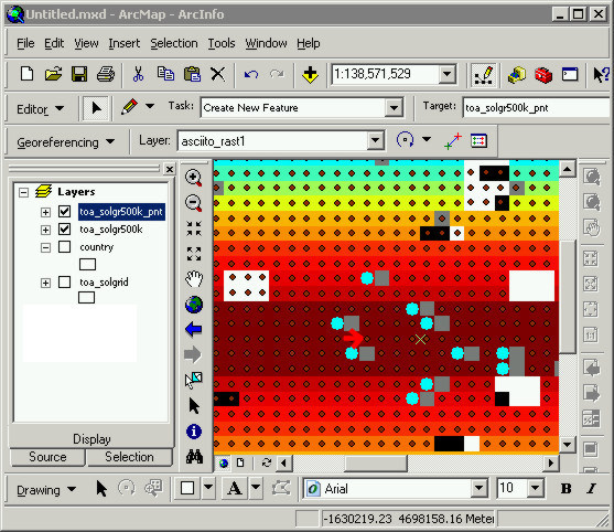
Below shows a more complicated pattern. Don't forget about the magic Undo button (Ctrl Z, or Edit -> Undo). Remember, only copy values along rows.
Select a set of points, copy-past right on top of the points you selected.
Slide the copy-pasted points that are selected over to fill-in the empty cells.
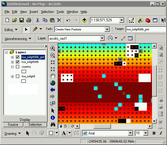
Select a pattern of single points by holding down Shift, Copy-Paste the selected points.
Slide over the copy-pasted group of points over to fill the empty spaces.
After you've finished filling in all the empty cells, expand the lattice horizontally by about 2 or 3 columns of points to the East and to the West. Select the entire right-hand side of points and copy-paste it, slide it over to expend the row by on cell width to the right. Copy-paste another entire column of points and expand the lattice to the right about 2 or 3 columns. Do the same thing for the Western side, expand the lattice to the left by 2 or 3 columns as well.
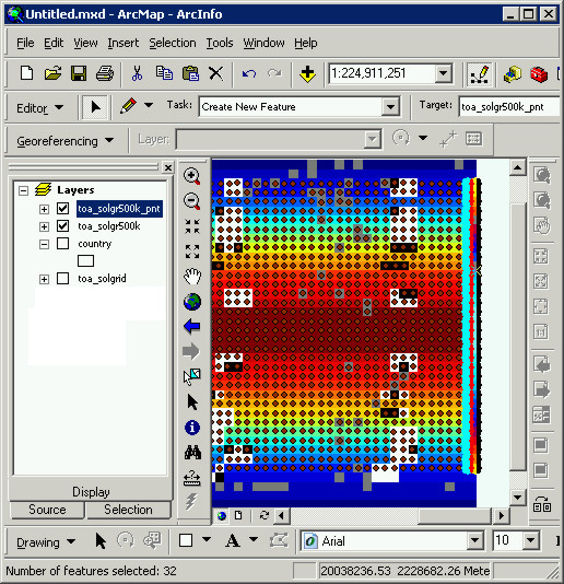
Click on the Editor button and from the pulldown menu choose Save Edits. Don't worry if your points are not perfectly aligned, they need to be close but not perfect.
Step 6.2 - Clean the Attribute Table
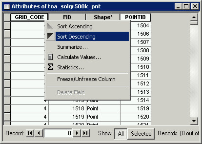
Each point is linked to an entry in a table, each point has a GRID_CODE value assigned to it. Look at the Attribute Table for toa_solgr500k_pnt, right-click on the data layer in ArcMap and choose Open Attribute Table. Sort the GRID_CODE column in Descending order by right-clicking on it.
If there are GRID_CODE values less than 4, get rid of those points. To select the GRID_CODE values less than 4, go to Selection at the top of ArcMap, and pull down to Select By Attribute. Make a query for "GRID_CODE" < 4, and click Apply. If there are any selected, delete them (go up to Edit -> Delete).
Click on the Editor button and from the pulldown menu choose Save Edits. Click on the Editor button again and from the pulldown menu select Stop Editing.
If ever you find yourself slaving over a complicated editing task, it helps to make a backup every once in a while. Occasionally, but rarely, a dataset may become corrupt for some reason (a glitch in the file system caused by a harddisk error, ArcGIS crashes in the middle of an editing session, the power goes out, or a butterfly farts in Tibet ... whatever). Just follow this procedure and you will save yourself the agony of having to redo hours of tedious work. I realize this sentence is almost pointless because this is something you will have to learn on your own, I just hope it doesn't cost you your job (or your sanity!). Save frequently, and always make backups.
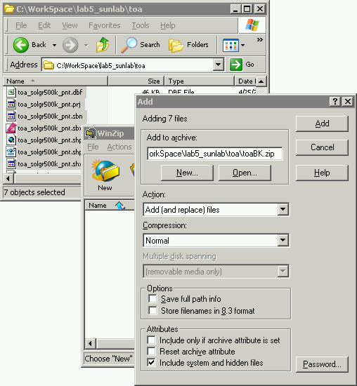
Open Windows Explorer and go to your lab5 folder. To backup the toa_solgr500k_pnt shapefile select all the component files, there are 7 of them, that constitute the shapefile (they all have the same name, but different file extensions). Right-click and choose Add to Zip. Name the output file with a capital BK on the end so you know what it is, and make sure the .zip file extension is on the end. (See Lab 5.1 Write-up)
Now we're safe from the butterflies, and we can do what we please.
Step 8 - Query to find the correct TOA values
The GRID_CODE attribute allows you to select a line (row) of points, this row of points represents a specific band of TOA value of Watts per square meter (W/m^2) at the top of the atmosphere. We need to figure out what GRID_CODE values for the points go with what TOA values from the TOA grid we rectified to fit the continent boundaries dataset.
First uncheck the resampled TOA grid, and check on the high resolution grid you can read. Go to the Editor button, and do Start Editing.
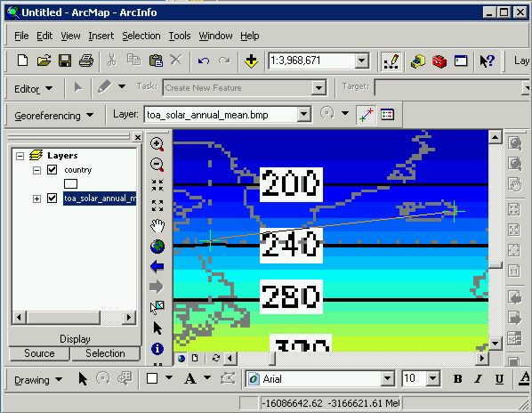
Go up to the Selection pulldown menu at the top of ArcMap and do Select By Attribute. Put in the query "GRID_CODE" = 4 and click Apply. Zoom in to see the selected row of point so you can read the text underneith. Notice in the screenshot below that this row of points falls more or less on the line marked with 200 W/m^2.

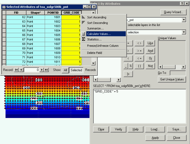
With that top row of points selected with 'GRID_CODE" = 4, right-click on the toa_solgr500k_pnt layer in ArcMap and choose Open Attribute Table.
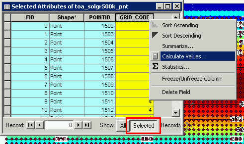
In the Attribute Table push the Selected button at the bottom so only the selected records are highlighted. To highlight the column of selected records click on the GRID_CODE heading at the top, they should turn yellow. Right-click on the GRID_CODE column heading and choose Calculate Values ...
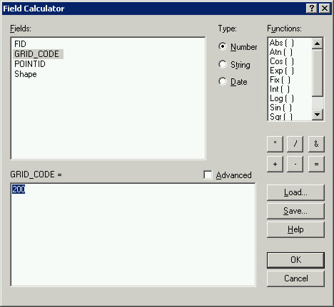
In the Calculate Values dialog type in 200 as shown below. This will "Calc" all the selected records in the attribute table (GRID_CODE = 4) to 200.
Do another Select By Attribute query for "GRID_CODE" = 5. Zoom in to look at the selected row of points. This time though you will have to estimate the TOA value because on the high resolution grid this row of point falls in between. Note the interval between the lines is 200-240, the row of points selected with "GRID_CODE" = 5 is about half way between 200 and 240.
Once you have determined the value, go back to the Attribute Table. Click the Selected button at the bottom and make sure the column is highlighted in yellow. Right-click on GRID_CODE, choose Calculate Values ... again, and type in the correct TOA value.
Now do Select By Attribute for "GRID_CODE" = 6 and Apply in the Select By Attribute dialog.
You can then do Zoom To Selected Features (also under the Selection pulldown menu) to see where that selected row of points is. Zoom in so you can see the values in the TOA grid are underneath the points. Notice that these are also 200, go back to the Attribute Table and to Calculate Values ... like you did before and put in 200, this will make all the points with GRID_CODE = 6, now 200. The Max value, from the original gif image, is 417 W/m^2. You can assign all of the points in the equatorial band (dark red) to this Max value.
Replace all of the GRID_CODE values in toa_solgr500k_pnt data layer using this procedure with the correct TOA values. After you're done, click on Editor -> Save Edits, then Stop Editing. Go up to Selection -> Clear Selected Features if any points are still selected.
Now for some error checking. We will be able to do this visually, the TOA values (GRID_CODE) should increase as you move North or South from the equatorial band.
Step 9 - Covert the lattice of points back to a grid, and resample
Now that we have a full lattice of points, each with the correct GRID_CODE attribute showing the W/m^2, we can make a clean grid out of it. The grid should be complete and extend far enough East and West so as to cover the full 360 degrees.
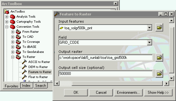
Start Toolbox, and go to Conversion Tools -> To Raster -> Feature to Raster. In the Feature to Raster dialog that opens input the point lattice you just got through editing, select Field as GRID_CODE, name the output "toa_grid500k", and set the Output cell size to 500,000.
The grid you converted from the points should automatically be added to ArcMap. Check to verify that all of the pixels are filled in, and the horizontal bars are filled in. If they are not you'll need to do Start Editing again and copy-paste points in to fill the gaps, and then convert the points to a grid again. Also check to verify that the values increase as you go north and south from the equator (you can do this using the Identfy tool to click on the grid).
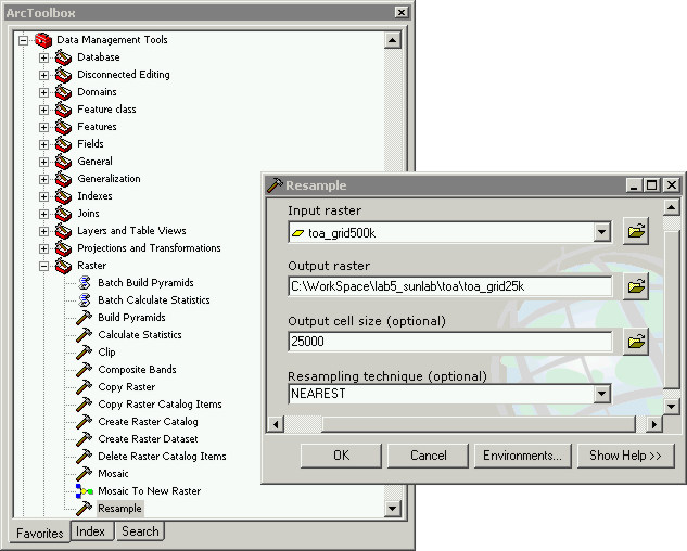
Once you have a grid completely filled-in Resample the grid cells (pixels) from 500000 to 25000. To resample a grid start Toolbox and go to Data Management Tools -> Raster -> Resample. In the Resample dialog set the input raster to toa_grid500k (the grid you created from the points), set the Output raster go to the toa folder and name it "toa_grid25k", in the Output cell size put 25000, then click OK.
Step 10 - Check the projection and export the final grid
You now have a grid of 25,000 pixels. Check the projection of the Data Frame (View -> Data Frame Properties, Coordinate Systems, Modify). The central meridian should be set to 0 (not 180) and the Linear Units should be set to Meter.
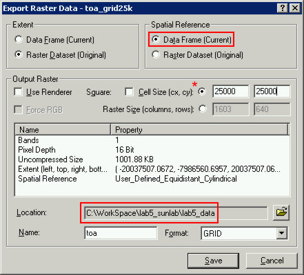
After you've check the coordinate system, and verified that it is set to Equidistant meters, go to Data -> Export Data.
In the Export Raster Data dialog set the Spatial Reference to Data Frame (Current), change the Cell size to 25000 x 25000, and change the output Location to be lab5_data. Name the output grid "toa".
After you have exported the final toa grid to lab5_data, make a map using this dataset you've just made.
Step 10 - Make a map of global TOA
We changed the Central Meridian of this projection in order to rectify the image file to geographic coordinates, now lets change it back to normal. Go back to View -> Data Frame Properties. Click the Modify button again and change the Central Meridian back to 0. Click Apply and OK.
Lets change the color scheme to something more agreeable with our eyes that also portrays what these data we just created represent.
Right-click on toa_grid25k, choose Properties, then Symbology. Choose Stretched from the options, and then find a Color Ramp that suits, you can check the Invert box to flip the around if it doesn't match the data values. Feel free to play around and change things, see how it looks, we are going to cover Data Classification specifically in a few weeks but you might find something you like just messing around for now.
Create a map layout with the continent boundaries, the final TOA grid from lab5_data, a 30 x 30 degree graticule, and a legend. The map should also have a title, your name, the data source, but you can also include a north arrow and a scalebar if you think they add cartographically to the map. Feel free to use your own color symbolization.
Continent outlines (continent.shp) can be found in this directory, C:\Program Files\ArcGIS\Bin\TemplateData\World\
Lab 5.1 Write-up (Include your TOA map with your write-up).
recreated by jeff 5/05, with help from ted