Start Windows Explorer, go to C:\WorkSpace\lab5. Go up to View -> Details, and list the contents

The raster (grid) you created from the point shapefile is actually a folder with files in it. Other files that are contained in another folder called "info" are associated with the files in the grid's folder. In Windows Explorer you can see this mysterious info folder. You cannot simply copy-paste these data (grids) like you can with all the component files the constitute a shapefile. This is a disadvantage of these formats.

Open the map layout you made for the TOA map for Lab 5.1. If ArcMap shows red exclamation marks because it can't find the data, right-click on the toa_grid500k layer, choose Properties, then under the Source tab there is a button called Set Data Source where you can locate the files ArcMap is wanting.

If the coordinate system for the Data Frame is not already set, set it with View -> Data Frame Properties -> Coordinate System to Plate Carree (WGS 1984). Right-click on the data layer in ArcMap and do Data -> Export Data. Under Spatial Reference in the Export Raster Data dialog, choose Data Frame (Current). This, as you know already, will make the data you export retain the projection information from this data (the new grid will have Plate Carree projection assigned to it).

Right-click on toa_grid500k, go to Data -> Export Data. In the dialog that opens, specify the Location as lab5_data. Name the new grid "toa", and select Data Frame (Current) for the Spatial Reference.

Before you close ArcMap, save the map layout in the lab5_data folder and name it appropriately. Once you've saved the map in lab5_data, right-click on the data layer, choose Properties, and under the Source tab, click on the Set Data Source button and tell ArcMap to use the TOA grid in the lab5_data folder you just exported.

Now that you've exported (copied) the TOA grid to the lab5_data folder, and made a new map layout with that data, lets clean up. Close ArcMap

Go back to Windows Explorer. Select everything in the lab5 folder except lab5_data. Right-click, choose Add to zip ... and make an archive called "lab5.1archive.zip". Be sure to check that the output path is in the lab5 folder and not within a folder below the current level of lab5_data, also make sure the .zip file extension is on the end.

After WinZip is done making lab5.1archive.zip, delete everything accept the lab5_data folder and lab5.1archive.zip. All you should have in the lab5 folder is the master data folder and the archive.zip file.

In the lab5_data folder there are two datasets, the TOA grid (and its associated info folder) and all the files that comprise the country shapefile. You should also have the TOA map layout somewhere, either in the lab5_data folder or somewhere else you can find it.

All clean, now we're ready to move on.

Step 2 - Get the climate data from NOAA

Climate and meteorological scientists are notorious for weird file formats. What we are about to do is download 12 data files, a global scale grid of cloudiness for each month of the year that was compiled from 31 years worth of weather station measurements. We are then going to convert these data files to grids and compute the average of the 12 as one final "average cloudiness" grid, we will also be making a "median cloudiness" grid. This will introduce you to the nightmare that is file format conversion. As with the gif we converted last time, I'm got just going to give you a ready made dataset - you're going to have to make it yourself! Although this time the data are real, not a gif, but they're in a strange format.

Go here: http://www.ngdc.noaa.gov/seg/cdroms/ged_iia/html/database.htm

Click on the Data Structure and Formats link above the list of datasets on the webpage linked above. In the Data Structure and Formats page, click on the Raster Grids link at the top. This will take you down that same page to a subsection titled, "Raster Grid (image/map) Data Files". In this section the data files themselves are explained (there are questions based on this material in the Lab 5.3 Write-up, and you will need to know some of these things to complete this lab).

Go back the main page (or click on the link above), and go to the webpage associated with the datasets titled "Leemans and Cramer IIASA Mean Monthly Values of Temperature, Precipitation, and Cloudiness on a Global Grid."

The IIASA dataset consists of three parts, we are only going to use the "Average Monthly "Cloudiness" (% sunshine)" part. But first we need to figure-out the basics: 1) What is the coordinate system? 2) What are the units? ("Spatial Representation" in their terms), 3) What is the "quantization" or "bit depth" ("Data Representation" in their terms)?

Other relevant things that you might want to know about these data later are what "Geographic Sampling" scheme was used? What technique was used to interpolate data values? What is the spatial accuracy? For now these questions are not important - make the data first and ask questions later!

Using Windows Explorer create a folder called "clouds" in the lab5 folder (not in the lab5_data folder, but at the same level in the directory structure as the lab5_data folder).

Windows Explorer by default makes little pictures/icons of things (like a Mac), but this is not useful if you're not looking at pictures. Change the view properties of Windows Explorer to show Details, and show file extensions.

To make Windows Explorer list the files and relevant info go up to the top and click on View -> Details, to make it show you the file extensions go up to Tools -> Folder Options. In the dialog that opens click on the View tab and uncheck "Hide extensions for known file types", then click Apply. To make this permanent for all the Windows Explorer windows you open click on the "Apply to All Folders" button. Click OK to close the Folder Options dialog. Now you will see files listed with their associated extensions along with file sizes.

Now download the data files. We are only going to be using the Average Monthly "Cloudiness" (% sunshine) component of IIASA dataset. Go down to the Cloudiness dataset (it has an image with a green background, and is towards the bottom of the IIASA webpage). Once you're there click on the link next to Projection called "latlong.ref". Notice they call the spheroid an ellipsoid, and they call the datum a spheroid. OK, fine, we can live with this. WGS84 is the spheroid for the Latitude/Longitude coordinate system they've used, and what is the projection listed here? (its in brackets) See Lab 5.2 Write-up.

Go back to the Cloudiness webpage again, and click on the link ".img" under Data in the table.

Clicking the link will take you to another page listing:

lccld01.doc
lccld01.img
.
.
.
lccld12.doc
lccld12.img

How big are the data files? How big are the other .doc files? One is < 1024 bytes one is > 1024 bytes (so it is labeled in Kilobytes, with a "K"). These files are small enough to download quickly. If instead of a K there was an M (or MB as is standard for megabyte), we would not be done downloading these files until tomorrow and the servers would probably not respond well to us all trying to download about a Gigabyte (GB, = 1024 MB) of data at the same time.

Right-click on the first .doc file, lccld01.doc, and choose Save Target As ..., and put this file into the clouds folder you made. They're not really Word documents as the .doc extension might make you to believe, don't try to open this file or Windows XP will think its a Word document and that'll cause problems.

Save only one of the .doc files, but save all 12 of the .img files into the clouds folder. A peculiar thing is that some installations of Windows XP for some reason will determine that these are mp3 files (and name them with the .mp3 file extension), this isn't an issue because we're going to change the file extension anyway. File extensions (.doc, .mp3, .bil) will tell the software you are trying to open them what they are, in some cases you can "fool the computer" by simply changing the file extension (but you have to have changed the Folder Options for Windows Explorer so it doesn't hide file extensions from you). See Lab 5.2 Write-up.

There should be 13 files in the clouds folder now, 12 with .img on the end, and 1 with .doc on the end. Now we need to change the file extensions so ArcGIS will recognize them for what they really are, generic binary data files. The extension .img refers to Erdas Imagine image files, kind of like the .doc refers to Word documents, but these are climate modeling people so we can forgive them for these details.

Here is a useful program for renaming lots of files. Download rename.exe from the link below

Right-click on 14aren.zip and do Save Target As ..., save it in the clouds folder.

http://www.1-4a.com/rename/download.htm

With Windows Explorer go to the clouds folder and unzip 14aren.zip, select only the executable "rename.exe" and click the Extract button, unzip it into the clouds folder (all you want is the executable, it has .exe on the end). Close winzip when you're done unzipping the program and run it.

When the program starts, change the setting to Whole Name and check on Replace (see red boxes below). Where you see the field with "this" in it, type in .img, and where you see the field with "by that" type in .bil. Rename.exe will show a before-and-after view of the right, if it looks right, click Start and it'll rename all the file extensions. You can click on Undo All if you mess up, but once you close rename.exe the changes are permanent.

Before you close rename.exe, push the F2 key (see orange box in the screenshot above) to see what all it'll do. This little program is not as simple as capture.exe, but it is extremely useful.

Close rename.exe when you're done check it out. We will not be using it again, I just wanted you to know about it incase you ever find yourself in a situation were you have to rename a lot of files. Most of the time there is an easier way, but whether or not the time you spend finding the "easy way" is justifiable in terms of how long it actually takes to complete a task is up to you.

Now that all the images have been renamed with .bil on the end instead of img, lets make a header file for the data files.

Go back to Windows Explorer, and now rename (the old fashion way) the first header file lccld01.doc to lccld01.hdr. To do this either click twice slowly to get the file's name editable, or right-click on the file and choose rename. Whatever you're comfortable with. Change the file extension from .doc to .hdr

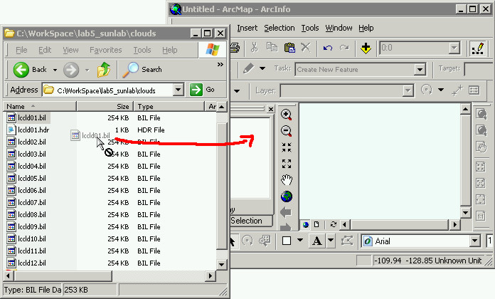
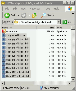
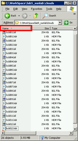
Right-click on the newly renamed lccld01.hdr, and choose Open With. If Notepad isn't an option in the Open With menu, find Notepad in the available programs. Click OK and Notepad should open showing you the header file's contents.

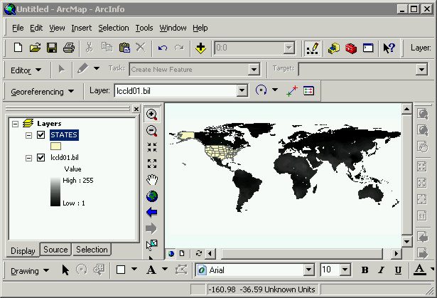
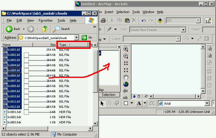
So what is a ASCII header file anyway? Yes it is techy jargon, but it also serves an important purpose. It will be used by ArcGIS to assign the data values contained in the data files (*.bil) you just downloaded and renamed. The header (lccld01.hdr) tells ArcGIS how big the output array is (rows/columns), what the coordinates are for grid's extent (upper left pixel's coordinate), how big the pixels are (cell dimensions), and a bunch of other things.

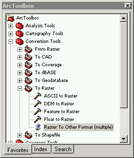
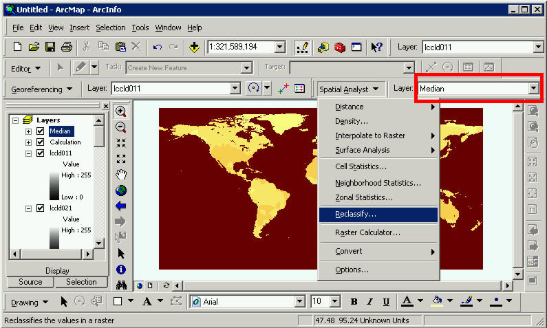
If you start ArcGIS Help and search for "float", and look at that "Float to Raster" help under the Usage tips. There you will find an example of the format for a floating point binary ASCII header that is wrong. We will not be using Workstation (you can thank me later), so we will be using the standard format for a header file.

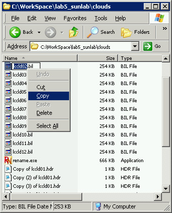
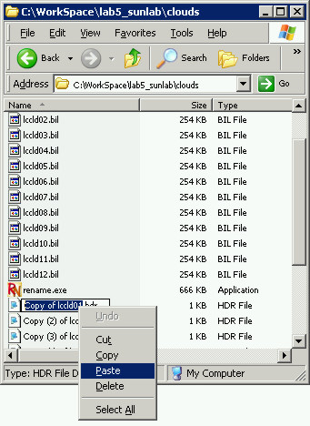
Go back to Notepad and delete everything in it, and Copy-paste the following into the header file. The appropriate format for a generic header, with some of the correct parameters for our data, is exactly as follows:

BYTEORDER I
LAYOUT BIL
NROWS
NCOLS
NBANDS 1
NBITS
BANDROWBYTES 720
TOTALROWBYTES 720
BANDGAPBYTES 0
NODATA 255
ULXMAP
ULYMAP
XDIM
YDIM

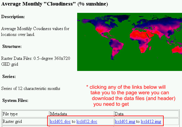
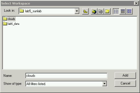
Now you need to put in the correct values for each of the parameters where the values are missing. To do this go back the website you downloaded the data from and try to find this information. Hint: it is under the "Data Structure and Formats" page, you're looking for something about Raster Metadata.

Link: http://www.ngdc.noaa.gov/seg/cdroms/ged_iia/html/database.htm

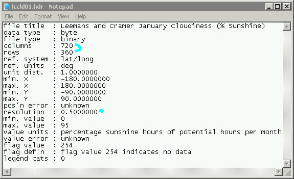
* Note that in the original header file (there is a screenshot of it above), that the order of the columns and row parameters is switched relative to what we want. You could reason your way through this though even if these parameters weren't labeled. If these data are in the latitude longitude coordinate system you know the resulting grid should be wider than it is tall (it should have more columns than rows right?). See Lab 5.2 Write-up.

BYTEORDER byte order in which image pixel values are stored

* Look at the "Data Structure and Formats", click on the "Numerical Types" link. Are the data in the file "big endian" or "little endian"? (See Lab 5.2 Write-up)
- Put an "M" for Motorola byte order (most significant byte first), "big endian"
- Put an "I" for IBM byte order (most significant byte last), "little endian"

LAYOUT organization of the bands in the file

* Put in "BIL" (stands for Band and Interleaved by Line, safest assumption for generic binary image format. There are also BSQ, BIP, but you will not see those often)

NROWS number of rows in the image
NCOLS number of columns in the image

NBANDS number of bands in the image

* Put in "1", our image only has one band

NBITS number of bits per pixel

* There are 8 bits in 1 byte, you read about this earlier in the "Data Structure and Formats" webpage under the "Raster Grid (image/map) Data Files" heading. (See Lab 5.2 Write-up)

BANDROWBYTES number of bytes per band per row

* = [ (number of pixels per row) * (bytes per pixel used to store data value for that pixel) ] Note: think about a grid, there are columns and rows, the number of pixels in a row is determined by the number of columns. In the data files we are using the data values are stored in 8-bit, 8 bits = 1 byte, so this parameter is 720. Make sense? (See Lab 5.2 Write-up)

TOTALROWBYTES total number of bytes of data per row

* this is the same as the BANDROWBYTES because these data files only have 1 band

BANDGAPBYTES

* Put "0" here. BIL has no gaps, there would be gaps for BSQ

NODATA value used for masking purposes

* Look at the screenshot of the original header file above, what is the "flag value"? Normally 255 would be standard practice because these data are "8-bit" (1 byte bit depth). Each bit is either 0 or 1, so there are 2^8 possible combinations of 0s and 1s, there are 0-255 possible 8-bit values. 255 is white, 0 is black.

ULXMAP longitude of upper-left pixel (in decimal degrees)
ULYMAP latitude of upper-left pixel (in decimal degrees)

* You should be able to figure these two out based on what you've learned already. "UL" stands for Upper Left, if these data are latitude longitude what is the upper left pixel's coordinate? (remember the negative/positive notation)

XDIM x dimension of a pixel in geographic units (in decimal degrees)
YDIM y dimension of a pixel in geographic units (in decimal degrees)

* "DIM" stands for dimension, the x-y resolution of the pixel

Congratulations, you've just made a ASCII header for a generic binary data file! I know, you're overwhelmed with joy.

One of the main difficulties with using data files like these in GIS is making different software (and operating systems) talk to each other and share data. File formats are the main problem with interoperability. For instance, when you get as an input the results from a sophisticated C program that was run on a UNIX server that models inputs from multiple points (say, 29 years of weather station records from around the world) and generates binary data files as outputs (of, say, % cloud cover per month) in arrays of values.

Our example here was relatively nice because the data were well described (legible metadata). There are situations were the data are not well described, or the metadata format make it difficult to find the parameters, or the parameters are incorrect. In these situations it basically boils down to trial-and-error, but if you know the basics of how a header file works you can usually reason your way though it and make it work.

After you've made the header file, save it, and then drag the lccld01.bil image data file from Windows Explorer into an empty ArcMap window. You don't have to drag it in, you can click the Add Data button if that is the way you prefer to do it. I just wanted you to know you can do it this way too, sometimes dragging a data file (or folder) in from Windows Explorer or ArcCatalog will work while the Add Data button will not. Don't ask me why, ArcMap is picky about what it will and will not open but if you drag it in it doesn't have a choice but to try to recognize the file.

When you try to open the .bil file with ArcMap it will automatically look for a .hdr header file. Don't fret because the image you see appears to be all black, get the Identify tool and click around (remember, the data values are percents as whole numbers).

Did the header file you made work? Move your cursor around the image and check to see if the coordinates look right (look at the coordinates in the lower-right of the ArcMap window).

Another way to check is to load some data we know are projected correctly with latitude longitude coordinates on top of it. In lab4.2 I gave you STATES that was projected with latitude/longitude coordinates, load that and see if it shows up in the correct place. You can also use the county.shp file in lab5_data.

If it doesn't look right, the coordinates are whacked, or the STATES don't show-up where they should, there is a problem with the header. You'll need to fix lccld01.hdr (ask me, I help).

Close ArcMap, and don't save the map.

What we have to this point is a folder called clouds with 12 identical binary data files that we renamed with .bil so ArcMap would recognize them as generic binary and know to look for a header.

Each of the data files contains average cloudiness for each month of the year for the world stored as an 8-bit value. We now need to make 12 identical header files that are named with the same name as the corresponding data file (each generic binary data file, .bil, should have a identical named header file to accompany it with the .hdr extension). We are going to do this by duplicating the good header that you just made and verified.

Copy-paste the header file you just made 11 times. After you do this, in Windows Explorer it should look like this (never mind that file size of rename.exe!)

Now rename each of the copies of the header file the old fashion manual way. To rename the files efficiently, clicking on the .bil file once, then click again, the name of the file should be editable now. Copy the name part, then click once, and then click again, on one of the copied .hdr file, paste the name you copied but make sure the .hdr file extension stays on the end.

Now that you've copied the text of the name you have it on your Windows clipboard. You can paste it again to another one of the copied lccld01.hdr files and rename it with "02.hdr" on the end, and then the next with "03.hdr" on the end.

You could make rename.exe do this using multiple copy-paste steps and different folders. Trust me though, its much easier to just do it the manual way. For simple things like file extensions, or adding numbers incrementally to the beginnings of file names, rename.exe is very efficient, but in this case it is not. If we were doing this for 30 or more files we'd figure out a way to make rename.exe do it.

Here are a series of screenshot describing visually the renaming process. Click once on the lccld02.bil file to select it, then click again to make the name editable. When mask out the file's name, right-click Copy (or Ctrl+C).

Next click once to select one of the copied lccld01.hdr files, then click again to make the name editable. Right-click and choose Paste (or Ctrl V).

Rename each of the copied lccld01.hdr files with the appropriate name. You want to make a lccld0#.hdr for each of the lccld0#.bil data files.

After you're done, you should have each data file named with .bil and then a .hdr file with the same file name in pairs. In Windows Explorer, click on the Name bar at the top of the list of files in Windows Explorer to sort alphabetically by name to check this.

We have now each data file named correctly, and a corresponding header file that generates a correct spatial representation of the data.

Step 4 - Convert BIL files to GRIDs

ArcMap if you try to add these bil files the conventional way by clicking the Add Data button, you can also just drag all the bil files into ArcMap. It will automatically look for the header files for each image, if there is a problem with one of your header files it will not load it.

Start ArcMap with an empty layout, list the data files in Windows Explorer by Type as shown below, then drag them into an empty ArcMap layout.

Now that we've made ArcGIS read in all the bil files, and we know that each header file works, lets make all the .bil files into grids.

Start Toolbox and got o Conversion Tools -> To Raster -> Raster To Other Format (multiple).

In the Raster to Other Format (multiple) dialog click on the folder button next to the Input Rasters field. Add all of the .bil files, next set the folder where the grids are to be written to. Click on the folder button next to the Output Workspace field, when you click the folder button the Select Workspace window will open where you need to choose the clouds folder. Navigate to where you can see the clouds folder, highlight it and click the Add button.

Set the Raster Format (optional) field to GRID. Click OK.

Go back to Windows Explorer and list the contents of the clouds folder by Name (click on the bar above the list of file names). Make sure there are 12 folders, remember that the GRID raster data structure actually consists of a folder with files in it, and these files are linked to other files stored in the info folder.

Now we are sure that we have each month's cloudiness (the percentage of cloud free days/month) in a usable GIS format, we are going to combine all of these grids.

Step 5 - Use Raster Calculator and Cell Statistics to make mean-median cloudiness grids

Start ArcMap and add all the grids you just made. You should use the Add Data button because ArcMap will see the grids as grids (not folders), but you could do this by dragging all the folders into ArcMap as well. Set the coordinate system of the new layout with View -> Data Frame Properties, go to Preferred -> Geographic Coordinate Systems -> World -> WGS 1984.

Right click on one of the grids and go to Properties, in the Source tab scroll down until you can see the Extent. Why is it -180.25, -89.75, 179.75, 90.25? (See Lab 5.2 Write-up)

Close the Layer Properties window and start the Spatial Analyst extension (this is one of the most powerful geoprocessing components of ArcGIS). Go to Tools -> Extensions, and check on Spatial Analyst. Click Close to exit the Extensions window. If a new toolbar didn't appear in the ArcMap window, turn on the Spatial Analyst extension's toolbar (View -> Toolbars, check on Spatial Analyst).

Click on the Spatial Analyst pulldown menu, and select Raster Calculator. All 12 of the open grids should be added to the Layers window of the Raster Calculator automatically. First add a open bracket at the very beginning, add the 1st grid by double clicking on it, then add a plus sign after it. See below.

Add the next grid by double clicking on it, then another plus sign, then the next grid and another plus sign ... When you have added all the grids put a close bracket on the end. Then click on the divide button in Raster Calculator and type in 12. It should not be hard to guess what you are about to do. What you have so far looks like the following.

Check to make sure you have brackets around the grids, and that you have all 12 grids. Then if all is well push the Evaluate button. The results should be automatically added to the ArcMap layout and called "Calculation".

Lets use a different Spatial Analyst tool to get Median percent cloudy days per year grids for the world. Click on the Spatial Analyst pulldown menu button again, this time choose Cell Statistics. In the Cell Statistic window highlight all the grids listed in the Layers frame, the click Add to move them all over to the Input rasters frame. In the Overlay statistics field, from the pulldown menu select Median. The click OK.

You should have two new grids in your ArcMap window now, one called Median and the other called Calculation.

This last step is important. Way back in the beginning when you were asked to read through the metadata and familiarize yourself with these data you probably saw mentioned in a few places "NODATA", you for sure saw it when you made the header file (you set it to 255). Well, although 255 is a good NoData value because it is distinct (it is the maximum possible data value for 8-bit data), it wreaks havoc on the statistics.

The data value 255 was used in the IIASA data files to represent pixels where there were no data. These pixels are those that occupy large lakes and the oceans. Now we are going to explicitly set 255 to NoData. The GRID raster data format supports NoData as a value, this is very important because it basically is a "mask" of the pixels were there are no data and it tells ArcGIS not to consider them.

Click on the Spatial Analyst pulldown menu button, set the Layer to Median (the grid you created using the Cell Statistics tool). Click the Spatial Analyst pulldown and select Reclassify.

In the Reclassify dialog click on the Unique button so it lists the unique values of the grid as whole numbers. Scroll down the list until you see 255 under the Old values column, to the right of it under the New values column click and type in "NoData" as shown in the screenshot below.

It will automatically add "Reclassify of Median" to the ArcMap layout. Next do Reclassify for the mean cloudiness grid you made with the Raster Calculator (its called Calculation). To do this change the Layer next to the Spatial Analyst pulldown menu button to Calculation, then click on the Spatial Analyst button and pull down to Reclassify. Click on the Unique button so it'll list the actual grid values, scroll down to 255 and type in NoData as you did before.

After you click OK, it'll automatically add "Reclass of Calculation" to your ArcMap layout. You now have two more new grids in your ArcMap layout, these are the keepers.

Right-click on the Reclass of Calculation (mean) grid in ArcMap and do Data -> Export Data.

Set the Spatial Reference to Data Source (Current), name the grid "cloud_mean", set the Location to lab5_data (use the folder button the highlight the lab5_folder, and click the Add button). Then click Save. No you do not want to add it to the layout, you will be starting a new map layout for the final maps.

Right-click on the Reclass of Median grid and Do Data -> Export Data. Name the Minimum grid "cloud_med". Use the same settings as before. Set the Spatial Reference as to Data Source (Current), set the output folder to be lab5_data.

After you have exported the two final grids (cloud_mean and cloud_med) into the lab5_data folder, close ArcMap. The temporary grids you generated with the Raster Calculator and Cell Statistics will be gone (they're still in some temp folder somewhere taking up diskspace, ArcGIS is sloppy like that, but its irrelevant with datasets this small).

Step 6 - Make maps of global cloudiness

Make two separate maps showing average annual % of cloudless days and the median % of cloudless days. Show the Mean and Median cloudiness with the same color scheme. Add a 30 x 30 degree graticule, a legend, a title, a source, your name, and a scale bar/north arrow if you think it adds cartographically to the map. Please be creative, you do not need to reproduce what I did - or even use the same projection!

If you have an ArcMap layout for the TOA map you made for Lab 5.1 use that as a template for this map. Open the TOA map from Lab 5.1, and rename it by doing Save As ... and saving it as cloud_mean_map. Remove the TOA data layer and add cloud_mean.

You will have to get rid of the old legend and Insert a new legend for this data after you have done Classify (described below). Once you've applied the Classified color symbology, you can modify the legend by selecting it, right-click and choose Convert to graphics, then you can ungroup and modify it as you want (but it is no longer linked to the data so if you decide to change the color symbolization you'll have to recreate the legend). After you're done tinkering around with the cloud_mean_map, save it, and then do Save As ... again and name it cloud_median_map. You can keep the same colors by just changing the data source (right click on cloud_mean in the map you just did Save As ... and named cloud_median_map, choose Properties, then go to the Source tab and click on Set Data Source, select the cloud_med grid. Then rename the layer in the ArcMap layout cloud_med (to avoid confusion). This way you can keep everything exactly the same and just use a different data layer.

Make two map using Classified for cloud_med and cloud_mean. In the Symbology tab click on the Classify button, in the Classification window next to Method selected Equal interval and set the number of classes to 10. Click OK and Apply.

Step 7 - Clean up

You're done-done, you've made the final maps, you have the two final cloudiness grids in lab5_data, and two ArcMap layouts for them.

Now lets do what we did for all the Lab 5.1 (TOA) droppings, WinZip everything and forget about it. This time all the files you need to archive are stored in the clouds folder. In Windows Explorer, right-click on the clouds folder and choose Add to Zip. For the sake of consistency name it lab5.2.archive.zip

Your workspace should be nice and organized now.

In the la5_data folder there are only the final versions of the files that you want and the map layouts you've made.

To be safe it might be a good idea to backup this lab5_data folder, but I will leave that up to you. Staying organized is half the battle and if you've made it to this point you've won (for today!).

Lab 5.3, which we will start on Thursday, will be about global population density and topography, but these data will be much easier to deal with (I promise). If you need help please don't hesitate to ask me. I will make myself available at a convenient time for you, 235 Hunt is open from 5-9:00 PM every day accept Friday and Saturday.